# 安装必要的包
if (!requireNamespace("ComplexHeatmap", quietly = TRUE)) {
  BiocManager::install("ComplexHeatmap")
}
if (!requireNamespace("circlize", quietly = TRUE)) {
  install.packages("circlize")
}
if (!requireNamespace("data.table", quietly = TRUE)) {
  install.packages("data.table")
}
if (!requireNamespace("dplyr", quietly = TRUE)) {
  install.packages("dplyr")
}

# 加载包
library(ComplexHeatmap)
library(circlize)
library(data.table)
library(ggplot2)
library(dplyr)单细胞 CNV 推断图
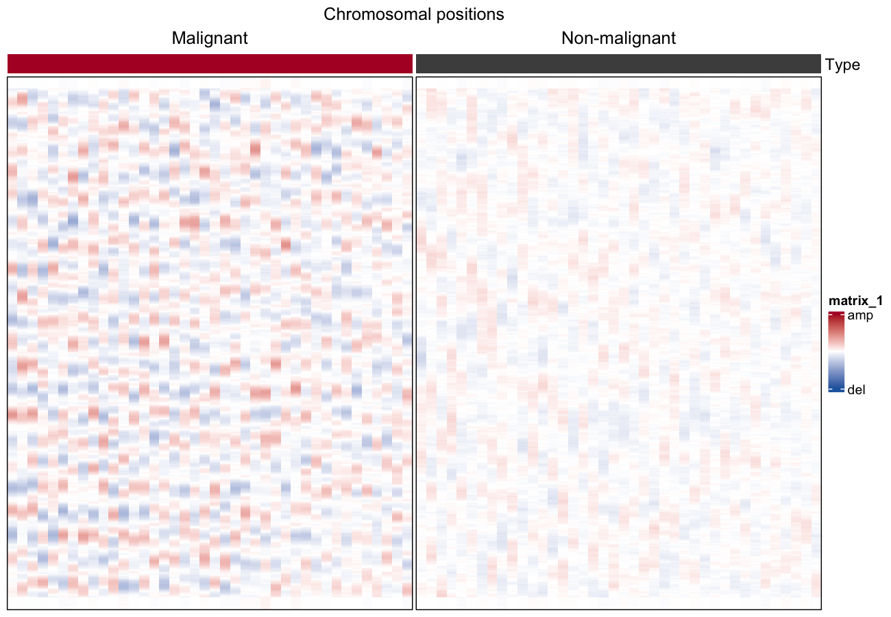
大尺度拷贝数 aberration 可以从单细胞 RNA-seq 推断:按基因组位置排序基因、在 100 基因窗口上平滑表达、对每个细胞做中位数中心化,剩余的波动就是 CNV 图景 [1]。把细胞(行)对染色体位置(列)铺开即可区分恶性与非恶性细胞,每细胞 CNV 评分用作排序统计量。
Example
Setup
系统要求:跨平台(Linux/MacOS/Windows)
编程语言:R
依赖包:
ComplexHeatmap;circlize;data.table;dplyr
sessioninfo::session_info("attached")─ Session info ───────────────────────────────────────────────────────────────
setting value
version R version 4.6.2 (2026-10-29)
os Ubuntu 26.04.1 LTS
system x86_64, linux-gnu
ui X11
language (EN)
collate C.UTF-8
ctype C.UTF-8
tz UTC
date 2026-11-05
pandoc 3.7.0.2 @ /usr/bin/ (via rmarkdown)
quarto 1.11.9 @ /usr/local/bin/quarto
─ Packages ───────────────────────────────────────────────────────────────────
! package * version date (UTC) lib source
P circlize * 0.4.18 2026-04-04 [?] RSPM
P ComplexHeatmap * 2.28.0 2026-04-28 [?] Bioconductor 3.23 (R 4.6.2)
P data.table * 1.18.6.1 2026-08-24 [?] RSPM
P dplyr * 1.2.1 2026-04-03 [?] RSPM
P ggplot2 * 4.0.3.9000 2026-11-03 [?] Github (tidyverse/ggplot2@b638d65)
[1] /home/runner/.cache/R/renv/library/Bizard-5140bdc6/linux-ubuntu-resolute/R-4.6/x86_64-pc-linux-gnu
[2] /home/runner/work/_temp/Library
[3] /opt/R/4.6.2/lib/R/library
* ── Packages attached to the search path.
P ── Loaded and on-disk path mismatch.
──────────────────────────────────────────────────────────────────────────────Data Preparation
真实输入是带细胞元数据的 log2-TPM 单细胞矩阵(参考数据为 GSE103322 HNSCC)。我们模拟按 22 条染色体排序的 400 个基因与 80 个细胞:40 个携带宽幅 CNV 波的恶性细胞和 40 个无波动的非恶性细胞。
set.seed(1401)
n_chr <- 22; genes_per_chr <- 50; n_gene <- n_chr * genes_per_chr
n_mal <- 40; n_nor <- 40

gene_pos <- expand.grid(chr = seq_len(n_chr), idx = seq_len(genes_per_chr))
gene_pos <- gene_pos[order(gene_pos$chr, gene_pos$idx), ]
genes <- paste0("G", sprintf("%04d", seq_len(n_gene)))

cell_type <- factor(c(rep("Malignant", n_mal), rep("Non-malignant", n_nor)),
                    levels = c("Malignant", "Non-malignant"))
cells <- paste0(substr(cell_type, 1, 3), "_", sprintf("%03d", seq_len(2 * n_mal)))

expr <- matrix(rnorm(n_gene * length(cells), mean = 5, sd = 0.5),
               nrow = n_gene, dimnames = list(genes, cells))
## broad CNV waves in malignant cells: sinusoid per chromosome,
## amplitude and phase vary per cell
for (i in seq_len(n_mal)) {
  for (chr in seq_len(n_chr)) {
    amp   <- runif(1, 0.4, 1.0) * sample(c(-1, 1), 1)        # del or amp
    phase <- runif(1, 0, 2 * pi)
    idx   <- which(gene_pos$chr == chr)
    expr[idx, i] <- expr[idx, i] +
      amp * sin(seq_along(idx) / length(idx) * 2 * pi + phase)
  }
}

## gene ordering + centring + bounding (the reference recipe)
gene_order <- order(gene_pos$chr, gene_pos$idx)
expr <- expr[gene_order, ]
rela <- sweep(expr, 1, rowMeans(expr))
rela <- pmin(pmax(rela, -3), 3)
Visualization
1. 滑动均值平滑(100 基因窗口)
smoothed <- rela
for (c_idx in seq_len(ncol(rela))) {
  smoothed[, c_idx] <- data.table::frollmean(rela[, c_idx], n = 50, align = "center")
}
smoothed[is.na(smoothed)] <- 0
## per-cell median re-centring after smoothing (Patel et al., 2014)
smoothed <- sweep(smoothed, 2, apply(smoothed, 2, median))

cnv_score <- colMeans(smoothed^2)
col_order <- order(cell_type, -cnv_score)

col_fun <- circlize::colorRamp2(c(-1.5, 0, 1.5), c("#2166AC", "white", "#B2182B"))
row_ha <- HeatmapAnnotation(
  df = data.frame(Type = cell_type[col_order],
                  `CNV score` = cnv_score[col_order]),
  col = list(Type = c(Malignant = "#B2182B", `Non-malignant` = "#4D4D4D")),
  annotation_name_side = "left")

chr_breaks <- cumsum(table(gene_pos$chr[gene_order]))[-n_chr]

Heatmap(smoothed[, col_order], name = "CNV",
        top_annotation = row_ha,
        col = col_fun,
        cluster_rows = FALSE, cluster_columns = FALSE,
        show_column_names = FALSE, show_row_names = FALSE,
        column_split = cell_type[col_order], column_gap = unit(1, "mm"),
        border = TRUE,
        heatmap_legend_param = list(at = c(-1.5, 0, 1.5),
                                    labels = c("del", "", "amp"))) |>
  draw(column_title = "Chromosomal positions")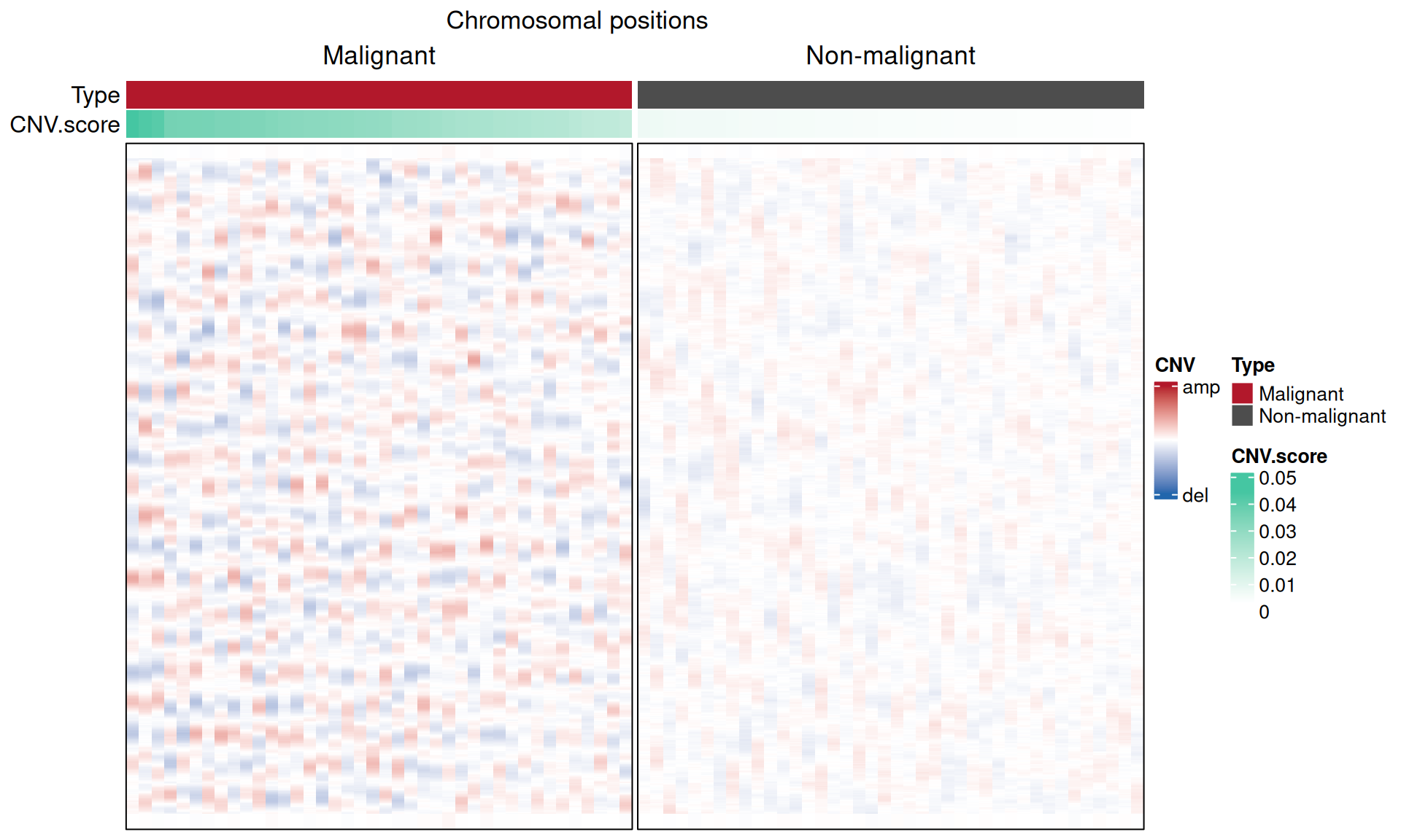
2. 依 CNV 评分区分恶性与非恶性
score_df <- data.frame(type = cell_type, score = cnv_score)
p_w <- wilcox.test(score ~ type, data = score_df)$p.value

ggplot(score_df, aes(type, score, fill = type)) +
  geom_boxplot(outlier.shape = NA, width = 0.55) +
  geom_jitter(width = 0.1, size = 0.8, alpha = 0.5, show.legend = FALSE) +
  scale_fill_manual(values = c(Malignant = "#B2182B", `Non-malignant` = "#4D4D4D")) +
  labs(title = sprintf("CNV score (Wilcoxon %s)",
       ifelse(p_w < 0.001, "p < 0.001", sprintf("p = %.3f", p_w))),
       x = NULL, y = "CNV score", fill = NULL) +
  theme_classic(base_size = 11) +
  theme(legend.position = "none")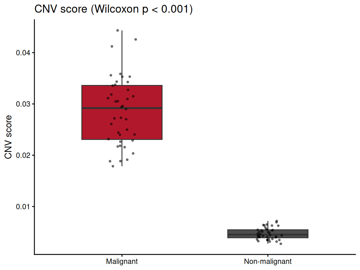
提示
Practice tips
- 推断 CNV 前先过滤低表达基因——近零表达会扭曲滑动均值、削弱波动。
- 按细胞(全部基因的中位数)中心化,而非按基因:波形是相对每个细胞基线的。
- CNV 评分兼作恶性判定——参考工作流用它标记 marker 基因漏掉的恶性细胞。
Application
推断 CNV 图景是肿瘤单细胞 RNA-seq(HNSCC、黑色素瘤、胶质瘤)的标准质控与恶性判定;热图通常是 scRNA-seq 肿瘤研究的第一张图。
Reference
[1] Puram SV, Tirosh I, Parikh AS, et al. Single-cell transcriptomic analysis of primary and metastatic tumor ecosystems in head and neck cancer. Cell. 2017;171(7):1611-1624.e24. doi:10.1016/j.cell.2017.10.044
[2] Xiaofan Lu, et al. FigureYa: A Standardized Visualization Framework for Enhancing Biomedical Data Interpretation and Research Efficiency. iMetaMed. 2025. doi:10.1002/imm3.70005