富集分析图（Python）

🤖 AI Skill — Download the Bizard unified skill for your AI assistant ⬇️ Download Skill ZIP

🔌 MCP Server — Let AI agents (Claude Code, Cursor, …) query Bizard live: claude mcp add bizard -- npx @openbiox/bizard-mcp — or the free hosted instance (no install, faster from mainland China): claude mcp add --transport http bizard http://biotree.top:38123/bizard-mcp/mcp 📖 MCP Docs

📖 Cite Bizard — if Bizard helps your research, please cite: Li, K., Zheng, H., Huang, K., et al. (2026). Bizard: A Community-Driven Platform for Accelerating and Enhancing Biomedical Data Visualization. iMetaMed, e70038. 🔗 DOI / BibTeX

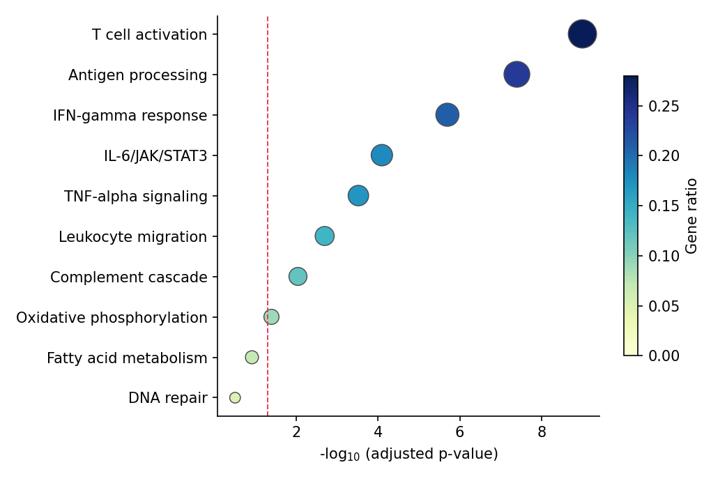
富集结果（GO/KEGG/reactome）通过两种标准图形阅读：按 −log10 校正 p 值排序的条形图，以及在条形基础上用点大小编码基因比例的点图。二者都是结果表之上的普通 matplotlib/seaborn 图层——同一配方适用于任何工具（gseapy、clusterProfiler 导出、ReactomePA）的输出。

示例

环境配置

• 系统要求：跨平台（Linux/MacOS/Windows）
• 编程语言：Python
• 依赖包：matplotlib、seaborn、pandas、numpy

import matplotlib.pyplot as plt
import seaborn as sns
import pandas as pd
import numpy as np

数据准备

我们模拟一个十条通路的富集表：通路名、基因数、比例与校正 p 值，按显著性排序——这些正是所有富集工具导出的列。

enrich = pd.DataFrame({
    'Pathway': ['T cell activation', 'Antigen processing', 'IFN-gamma response',
                'IL-6/JAK/STAT3', 'TNF-alpha signaling', 'Leukocyte migration',
                'Complement cascade', 'Oxidative phosphorylation',
                'Fatty acid metabolism', 'DNA repair'],
    'Count': [42, 35, 28, 24, 22, 19, 17, 12, 9, 6],
    'GeneRatio': [0.28, 0.24, 0.21, 0.18, 0.17, 0.14, 0.12, 0.09, 0.07, 0.05],
    'padj': [1e-9, 4e-8, 2e-6, 8e-5, 3e-4, 2e-3, 9e-3, 0.04, 0.12, 0.31],
})
enrich['NegLogP'] = -np.log10(enrich.padj)

可视化

排序条形图

按 −log10 padj 排序的横向条形，配显著性阈值线与数值标签，使图形自含。

top = enrich.sort_values('NegLogP')

fig, ax = plt.subplots(figsize=(6.8, 4.4))
ax.barh(top.Pathway, top.NegLogP, color='#8da0cb',
        edgecolor='0.25', linewidth=0.6)
for y, v in enumerate(top.NegLogP):
    ax.text(v + 0.06, y, f'{v:.1f}', va='center', fontsize=8.5, color='0.25')
ax.axvline(-np.log10(0.05), color='#e63946', linewidth=0.9, linestyle='--')
ax.text(-np.log10(0.05) + 0.06, -0.55, 'padj = 0.05', fontsize=8.5,
        color='#e63946')
ax.set_xlabel('-log$_{10}$ (adjusted p-value)')
ax.spines[['top', 'right']].set_visible(False)
plt.tight_layout()
plt.show()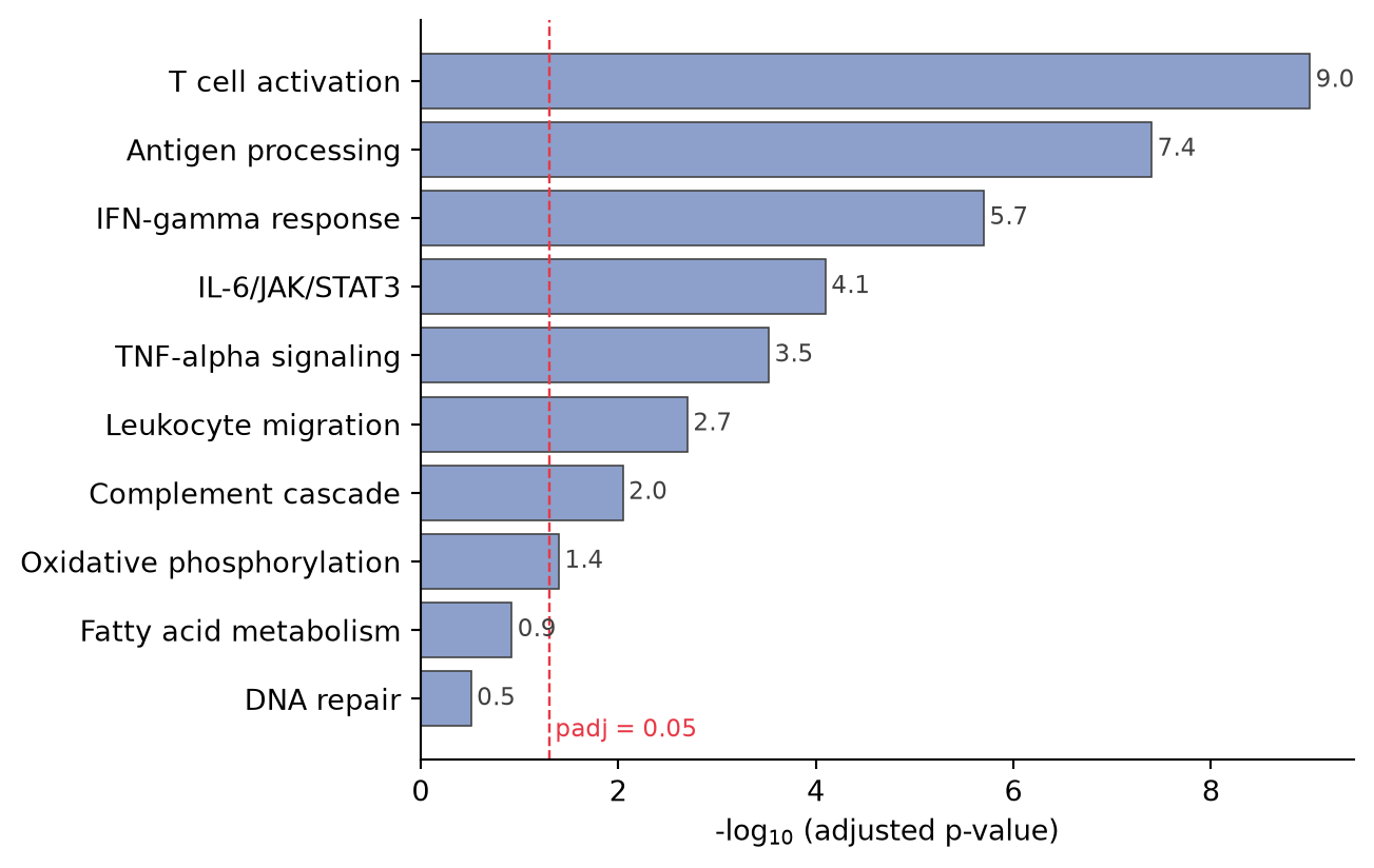

图 1: 按 -log10 校正 p 值排序的富集通路条形图

带基因比例的点图

点图引入第三变量：点大小为基因数，颜色为基因比例——clusterProfiler 推广的格式。

top = enrich.sort_values('NegLogP')

fig, ax = plt.subplots(figsize=(6.8, 4.6))
sc = ax.scatter(top.NegLogP, top.Pathway, s=top.Count * 9,
                c=top.GeneRatio, cmap='YlGnBu', edgecolor='0.3',
                linewidth=0.7, vmin=0, vmax=top.GeneRatio.max())
cb = fig.colorbar(sc, ax=ax, shrink=0.7)
cb.set_label('Gene ratio')
ax.axvline(-np.log10(0.05), color='#e63946', linewidth=0.9, linestyle='--')
ax.set_xlabel('-log$_{10}$ (adjusted p-value)')
ax.spines[['top', 'right']].set_visible(False)
plt.tight_layout()
plt.show()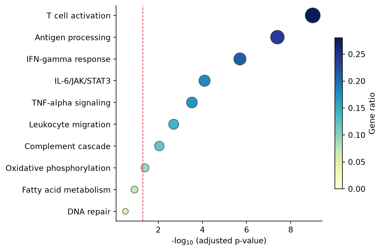

图 2: 富集点图：颜色编码比例，大小编码基因数

参考文献

1. Yu, G., Wang, L. G., Han, Y., & He, Q. Y. (2012). clusterProfiler: an R package for comparing biological themes among gene clusters. OMICS, 16(5), 284-287.
2. Hunter, J. D. (2007). Matplotlib: A 2D graphics environment. Computing in Science & Engineering, 9(3), 90-95.