if (!requireNamespace("ggplot2", quietly = TRUE)) install.packages("ggplot2")
if (!requireNamespace("dplyr", quietly = TRUE)) install.packages("dplyr")

library(ggplot2)
library(dplyr)RNA 速率图
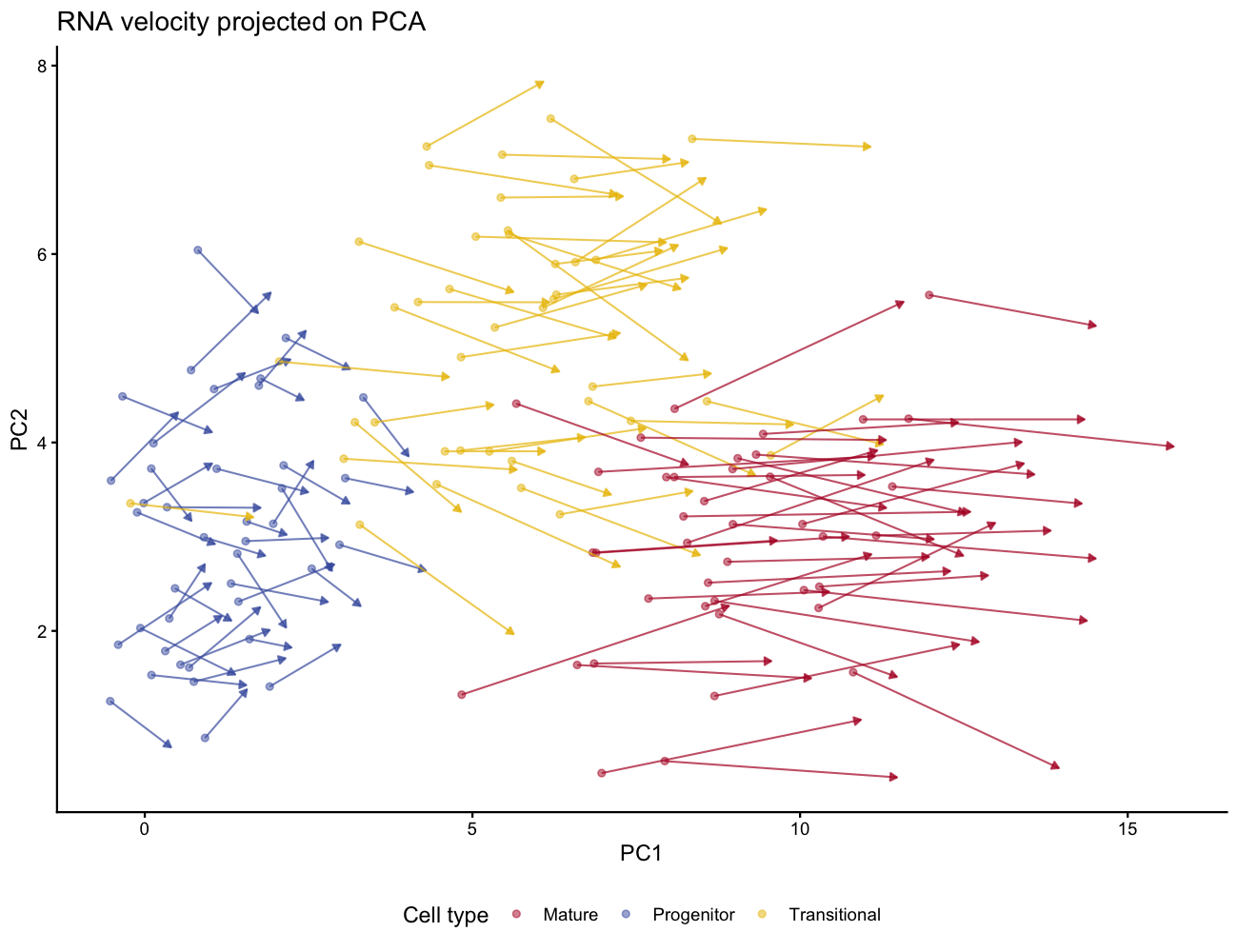
RNA 速率——基因表达的时间导数——从单细胞 RNA-seq 中的未剪接与剪接 mRNA 比值估计 [1]。经典配图将速率箭头投影到低维嵌入(PCA 或 UMAP)上:箭头越长表示预测的转录活性越高。本教程模拟速率数据并用 geom_segment() + arrow() 绘制箭头图。
Example
Setup
系统要求:跨平台(Linux/MacOS/Windows)
编程语言:R
依赖包:
ggplot2;dplyr
sessioninfo::session_info("attached")─ Session info ───────────────────────────────────────────────────────────────
setting value
version R version 4.6.2 (2026-10-29)
os Ubuntu 26.04.1 LTS
system x86_64, linux-gnu
ui X11
language (EN)
collate C.UTF-8
ctype C.UTF-8
tz UTC
date 2026-11-05
pandoc 3.7.0.2 @ /usr/bin/ (via rmarkdown)
quarto 1.11.9 @ /usr/local/bin/quarto
─ Packages ───────────────────────────────────────────────────────────────────
! package * version date (UTC) lib source
P dplyr * 1.2.1 2026-04-03 [?] RSPM
P ggplot2 * 4.0.3.9000 2026-11-03 [?] Github (tidyverse/ggplot2@b638d65)
[1] /home/runner/.cache/R/renv/library/Bizard-5140bdc6/linux-ubuntu-resolute/R-4.6/x86_64-pc-linux-gnu
[2] /home/runner/work/_temp/Library
[3] /opt/R/4.6.2/lib/R/library
* ── Packages attached to the search path.
P ── Loaded and on-disk path mismatch.
──────────────────────────────────────────────────────────────────────────────Data Preparation
真实数据中,velocyto.R 从剪接/未剪接计数计算细胞级速率矩阵,再将箭头投影到 PCA 或 UMAP 坐标。我们直接模拟该输出:沿分化轨迹排列的 3 个群共 120 个细胞,速率向量沿 PC1 正向指向前方。
set.seed(2501)
n_per <- 40
n_cell <- n_per * 3
cell_type <- rep(c("Progenitor", "Transitional", "Mature"), each = n_per)

pca1 <- c(rep(1, n_per), rep(5, n_per), rep(9, n_per)) + rnorm(n_cell, sd = 1.5)
pca2 <- c(rnorm(n_per, 3), rnorm(n_per, 5), rnorm(n_per, 3)) + rnorm(n_cell, sd = 0.5)

# velocity: points forward along PC1, magnitude increases with differentiation
vel_x <- c(runif(n_per, 0.5, 1.5), runif(n_per, 1.5, 3.0), runif(n_per, 2.5, 4.5))
vel_y <- rnorm(n_cell, sd = 0.5)

vel_df <- data.frame(PC1 = pca1, PC2 = pca2, cluster = cell_type,
                     vx = vel_x, vy = vel_y)
head(vel_df, 3)
PC1 PC2 cluster vx vy
1 0.809963 6.042075 Progenitor 0.9189087 -0.66934696
2 1.598161 1.912981 Progenitor 0.6415596 -0.08982668
3 1.412747 2.820119 Progenitor 0.7437892 -0.78530950Visualization
1. PCA 上的 RNA 速率箭头
ggplot(vel_df, aes(PC1, PC2, colour = cluster)) +
  geom_point(size = 1.5, alpha = 0.5) +
  geom_segment(aes(xend = PC1 + vx, yend = PC2 + vy),
               arrow = arrow(length = unit(0.15, "cm"), type = "closed"),
               linewidth = 0.5, alpha = 0.7, show.legend = FALSE) +
  scale_colour_manual(values = c(Progenitor = "#445EAD", Transitional = "#EABF00",
                                 Mature = "#B2182B")) +
  labs(x = "PC1", y = "PC2", colour = "Cell type",
       title = "RNA velocity projected on PCA") +
  theme_classic(base_size = 11) +
  theme(legend.position = "bottom")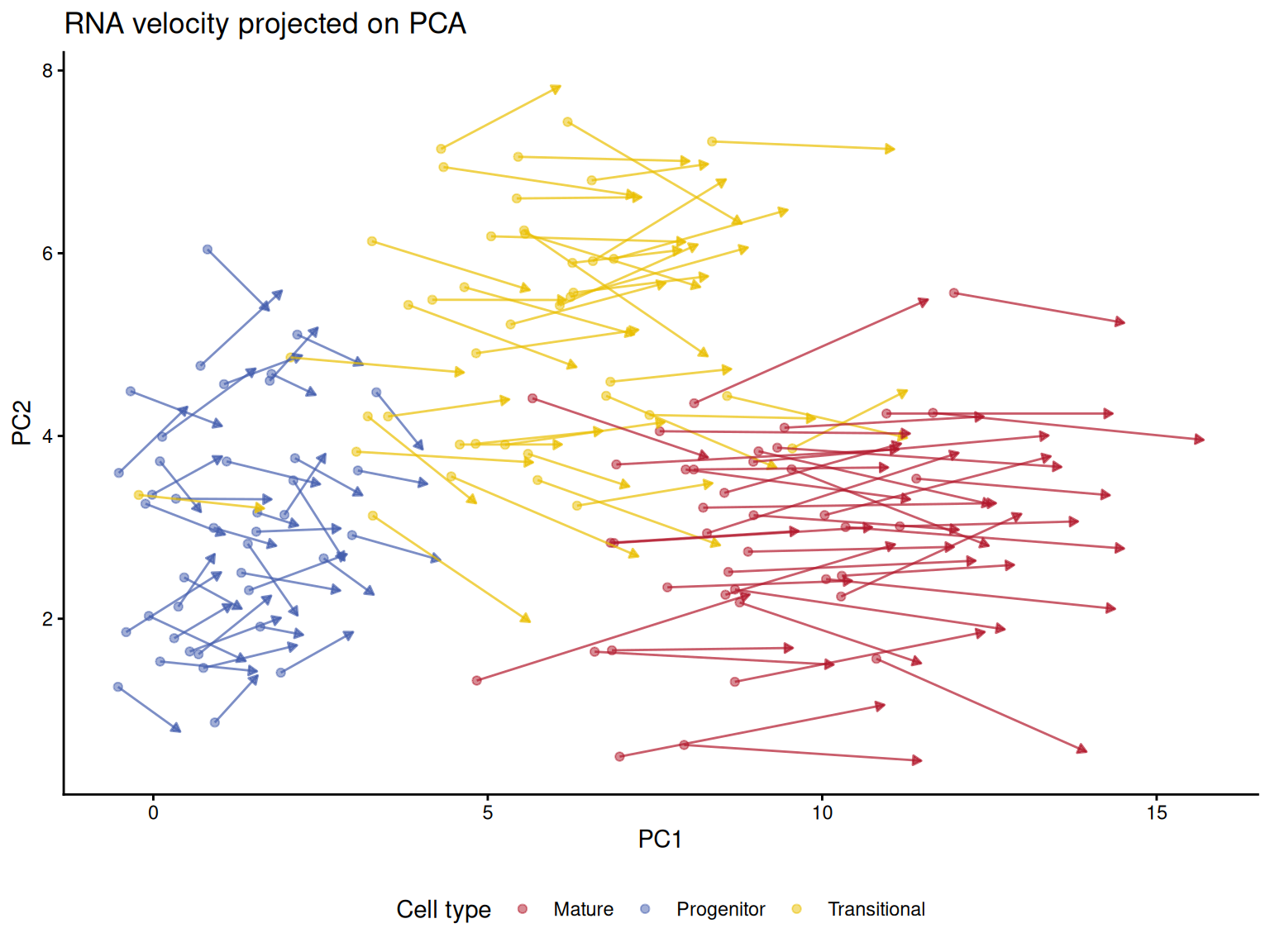
2. 各细胞类型的速率量级
vel_df$speed <- sqrt(vel_df$vx^2 + vel_df$vy^2)
p_kw <- kruskal.test(speed ~ cluster, data = vel_df)$p.value

ggplot(vel_df, aes(cluster, speed, fill = cluster)) +
  geom_boxplot(outlier.shape = NA, width = 0.55) +
  geom_jitter(width = 0.15, size = 0.6, alpha = 0.5, show.legend = FALSE) +
  scale_fill_manual(values = c(Progenitor = "#445EAD", Transitional = "#EABF00",
                               Mature = "#B2182B")) +
  labs(title = sprintf("Velocity magnitude (Kruskal-Wallis %s)",
       ifelse(p_kw < 0.001, "p < 0.001", sprintf("p = %.3f", p_kw))),
       x = NULL, y = "Velocity magnitude") +
  theme_classic(base_size = 11) +
  theme(legend.position = "none")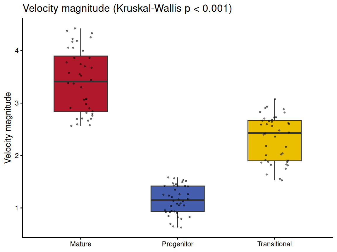
提示
Practice tips
- 速率箭头用
geom_segment()+arrow(length = unit(0.15, "cm"), type = "closed")——不同图幅下调整长度以保持可读性。 - 真实数据用
velocyto.R::gene.relative.velocity.estimates()计算速率矩阵,再用velocyto.R::show.velocity.on.embedding.cor()画内建箭头图;上方 ggplot2 配方提供更精细的美学控制。 - 用速度(
sqrt(vx^2 + vy^2))而非细胞类型给箭头着色,可突出转录活性高的区域。
Application
RNA 速率箭头是发育和肿瘤 scRNA-seq 研究中展示分化方向的标准配图。
Reference
[1] La Manno G, Soldatov R, Zeisel A, et al. RNA velocity of single cells. Nature. 2018;560(7719):494-498. doi:10.1038/s41586-018-0414-6
[2] Xiaofan Lu, et al. FigureYa: A Standardized Visualization Framework for Enhancing Biomedical Data Interpretation and Research Efficiency. iMetaMed. 2025. doi:10.1002/imm3.70005