# 安装包
if (!requireNamespace("ComplexHeatmap", quietly = TRUE)) {
  BiocManager::install("ComplexHeatmap")
}
if (!requireNamespace("dendextend", quietly = TRUE)) {
  install.packages("dendextend")
}
if (!requireNamespace("tidyr", quietly = TRUE)) {
  install.packages("tidyr")
}
if (!requireNamespace("circlize", quietly = TRUE)) {
  install.packages("circlize")
}
if (!requireNamespace("gridExtra", quietly = TRUE)) {
  install.packages("gridExtra")
}
if (!requireNamespace("pheatmap", quietly = TRUE)) {
  install.packages("pheatmap")
}

# 加载包
library(ComplexHeatmap)
library(dendextend)
library(tidyr)
library(circlize)
library(gridExtra)
library(pheatmap)复杂热图
示例
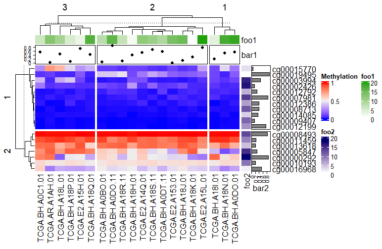
复杂热图(Complex Heatmap)是一种高级数据可视化工具,主要用于展示多维数据的矩阵关系,并在基础热图(Heatmap)上增加了多层次注释、聚类分析、数据拆分等功能。它能够更清晰地呈现复杂数据的内在结构和关联性。
环境配置
系统要求: 跨平台(Linux/MacOS/Windows)
编程语言:R
依赖包:
ComplexHeatmap,dendextend,tidyr,circlize,gridExtra,pheatmap
sessioninfo::session_info("attached")─ Session info ───────────────────────────────────────────────────────────────
setting value
version R version 4.6.2 (2026-10-29)
os Ubuntu 26.04.1 LTS
system x86_64, linux-gnu
ui X11
language (EN)
collate C.UTF-8
ctype C.UTF-8
tz UTC
date 2026-11-05
pandoc 3.7.0.2 @ /usr/bin/ (via rmarkdown)
quarto 1.11.9 @ /usr/local/bin/quarto
─ Packages ───────────────────────────────────────────────────────────────────
! package * version date (UTC) lib source
P circlize * 0.4.18 2026-04-04 [?] RSPM
P ComplexHeatmap * 2.28.0 2026-04-28 [?] Bioconductor 3.23 (R 4.6.2)
P dendextend * 1.19.1 2025-07-15 [?] RSPM
P gridExtra * 2.3.1 2026-06-25 [?] RSPM
P pheatmap * 1.0.13 2025-06-05 [?] RSPM
P tidyr * 1.3.2 2025-12-19 [?] RSPM
[1] /home/runner/.cache/R/renv/library/Bizard-5140bdc6/linux-ubuntu-resolute/R-4.6/x86_64-pc-linux-gnu
[2] /home/runner/work/_temp/Library
[3] /opt/R/4.6.2/lib/R/library
* ── Packages attached to the search path.
P ── Loaded and on-disk path mismatch.
──────────────────────────────────────────────────────────────────────────────数据准备
数据主要来自TCGA数据库的甲基化数据
#data_mat(连续型)
data <- readr::read_csv("https://bizard-1301043367.cos.ap-guangzhou.myqcloud.com/TCGA.BRCA.sampleMap_HumanMethylation27_ch.csv")

data <- as.data.frame(data)
rownames(data) <- data[,1]
data <- data[,-1]

data_TCGA <- na.omit(data[1:20,1:20])

data_TCGA <- as.matrix(data_TCGA)

#离散型
discrete_mat = matrix(sample(1:5, 100, replace = TRUE), 10, 10)
可视化
1. 基础复杂热图
连续型变量
这里我们以TCGA数据库的甲基化数据为例
# 连续型变量
Heatmap(data_TCGA , name = "Methylation")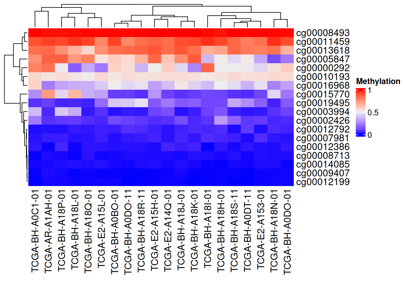
上图为甲基化水平的复杂热图,列为基因位点,行为样本。红色表示高甲基化水平,蓝色表示低甲基化水平。边轴为聚类分析结果。
离散型变量
这里我们以生成数据为例
# 离散型变量
Heatmap(discrete_mat,  name = "mat")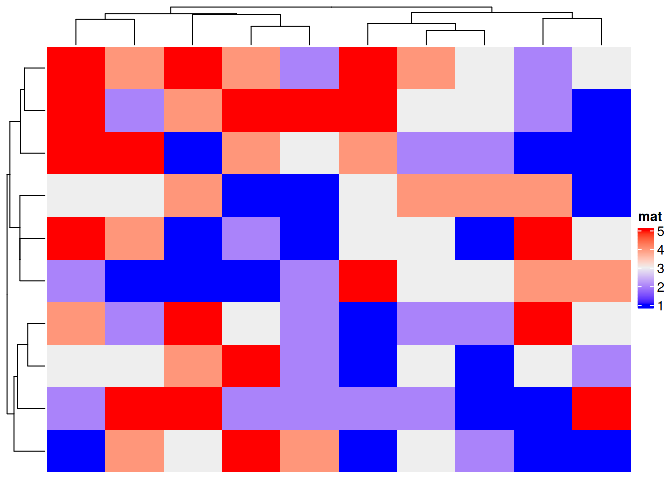
上图为生成的离散变量的复杂热图,边轴为聚类分析结果。
2. 个性化
2.1 颜色自定义
连续型变量
# 连续型变量颜色自定义
col_fun = colorRamp2(c(0, 0.5, 1),  #设置截断点
                     c("blue", "white", "pink"))
Heatmap(data_TCGA, name = "Methylation", col = col_fun,
              column_title = "自定义三段颜色")
# 连续型变量颜色自定义
Heatmap(data_TCGA, name = "Methylation", col = rev(rainbow(10)),
        column_title = "创建颜色向量")
离散型变量
# 离散型变量颜色自定义
colors <- c(
  "1" = "#BBEDA7",
  "2" = "#F3D8FA",
  "3" = "#FFECA1",
  "4" = "#D9E6F7",
  "5" = "#EFBEC6"
)
Heatmap(discrete_mat, name = "mat", col = colors,
        column_title = "离散型变量颜色自定义")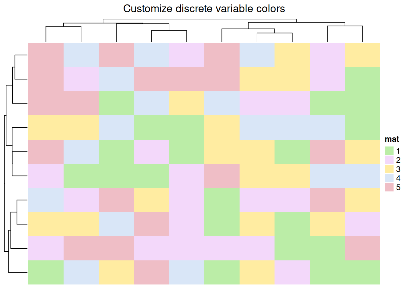
2.2 边框自定义
# 边框自定义
Heatmap(data_TCGA, name = "Methylation",
        border = "black", #border值可为FALSE或者颜色
        rect_gp = gpar(col = "white", lwd = 2),#lty线型, lwd线宽
        column_title = "边框自定义")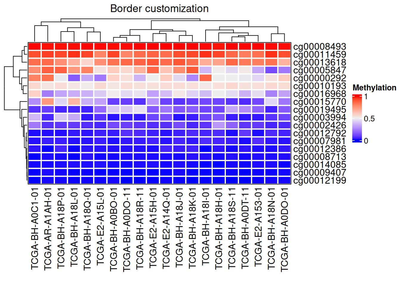
3. 聚类
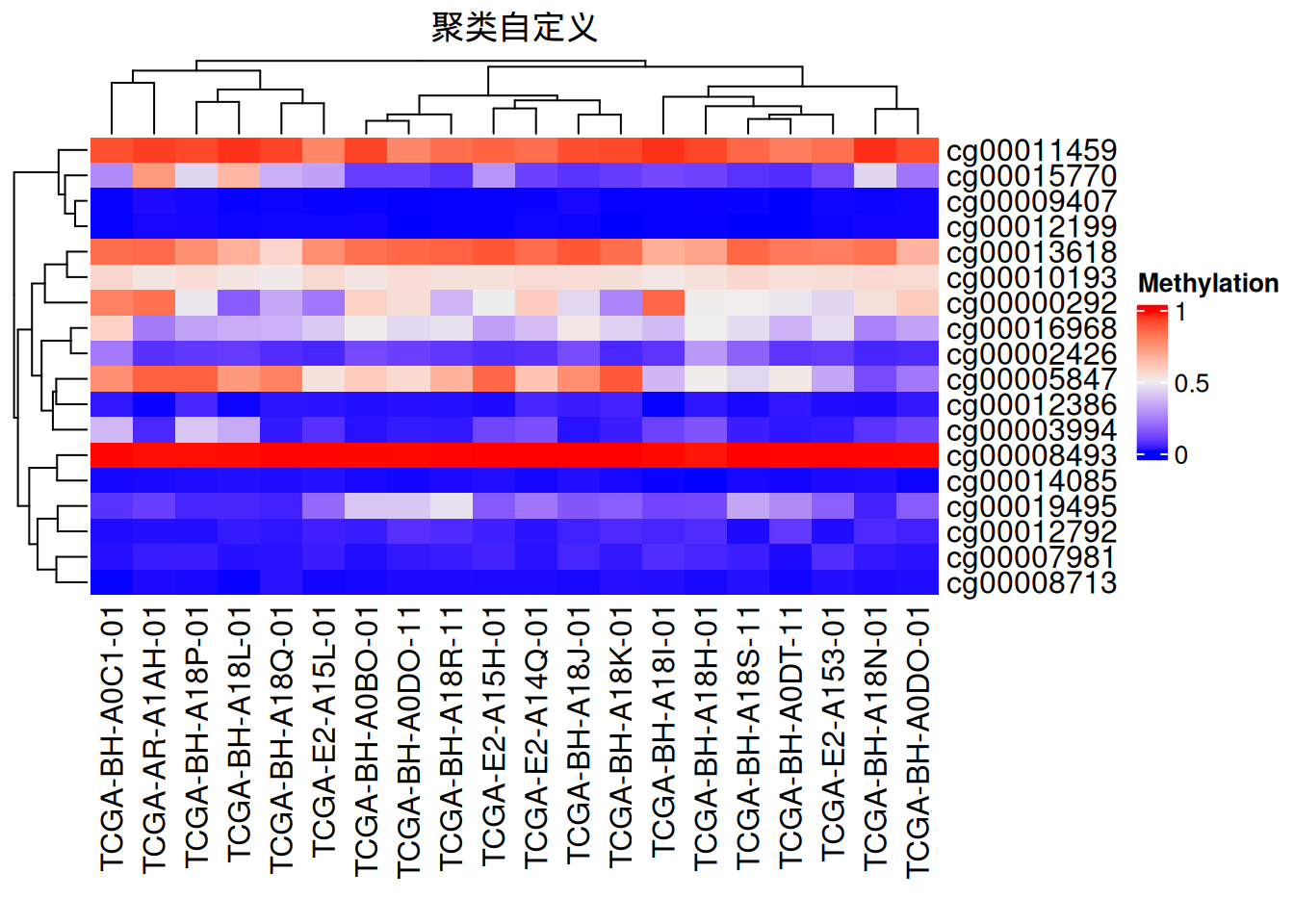
可以自定义聚类方法,树状图位置、大小等
# 聚类
Heatmap(data_TCGA, name = "Methylation",
       # row_dend_side = "right",
       # column_dend_side = "bottom", #可调整树状图位置
        column_dend_height = unit(1, "cm"),
        row_dend_width = unit(1, "cm"),#可调整树状图距离
        column_title = "聚类自定义",
        clustering_distance_rows = "pearson", #聚类方法,可自设函数
      # show_parent_dend_line = FALSE  #可隐藏虚线
) 
树状图渲染
我们还利用dendextend包对树状图进行颜色渲染
# 树状图渲染
row_dend = as.dendrogram(hclust(dist(data_TCGA)))
row_dend = color_branches(row_dend, k = 2)  #生成分支
#数字表示颜色数量
Heatmap(data_TCGA, name = "Methylation",
        cluster_rows = row_dend,
      # row_dend_gp = gpar(col = "red")  #也可自定义颜色
        )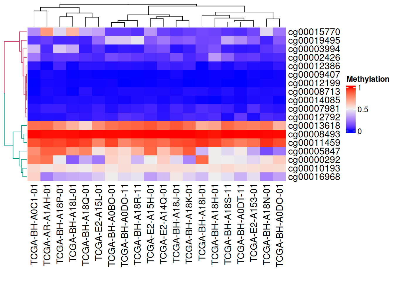
上图可见树状图分支为不同颜色
4. 分割
连续型变量
采用k-means聚类分割
# 连续型变量分割
Heatmap(data_TCGA,
        name = "Methylation",
        row_km = 2,  #设置分割数
        column_km = 3)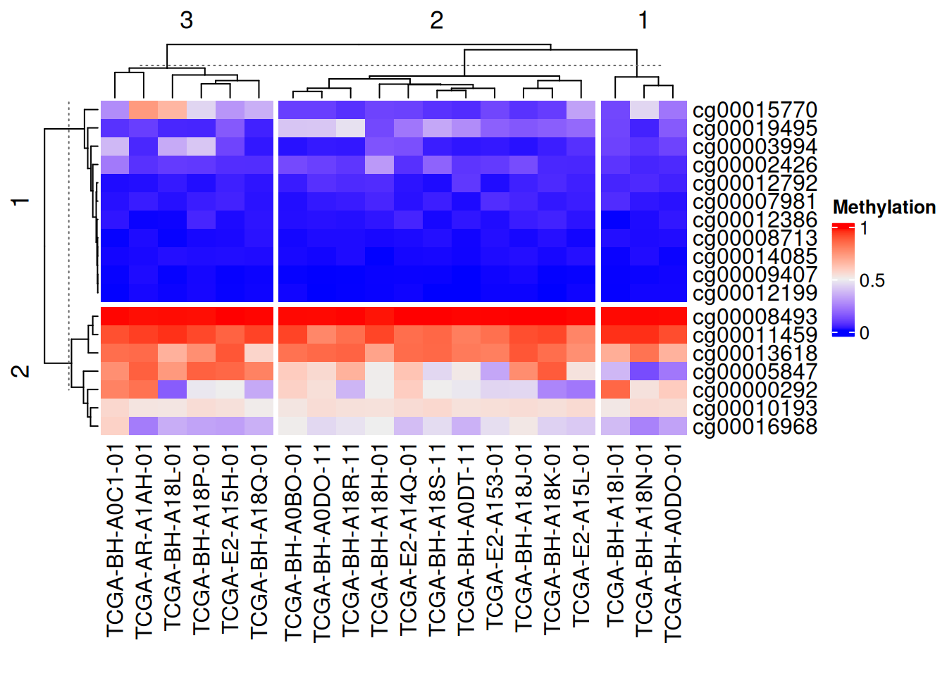
利用向量分割
# 利用向量分割
Heatmap(data_TCGA, name = "Methylation",
        row_split = rep(c("A", "B"), 9),
        column_split = rep(c("C", "D"), 10))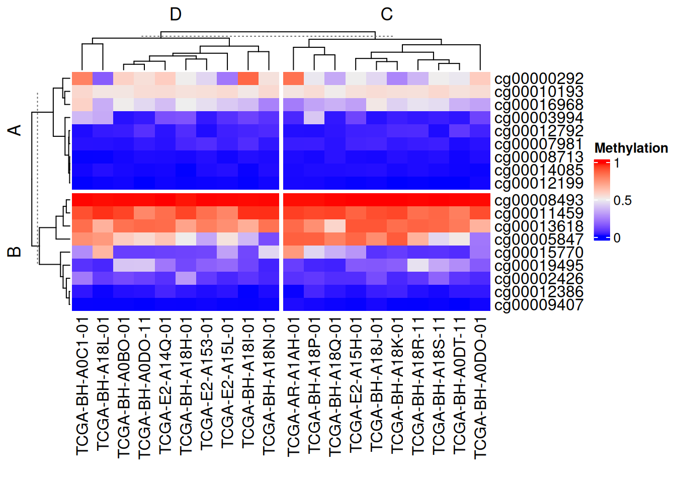
利用矩阵分割
# 利用矩阵分割
Heatmap(data_TCGA, name = "Methylation",
        row_split = data.frame(rep(c("A", "B"), 9),
                               rep(c("C", "D"), each = 9)))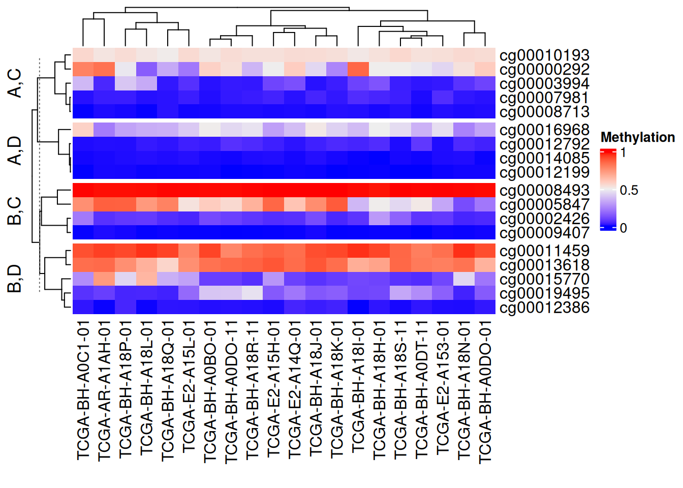
以上分割方法均可行列独立混使用,设置show_parent_dend_line = FALSE可隐藏虚线
离散型变量
按指定行列进行分割
# 按指定行列进行分割
Heatmap(discrete_mat,
        name = "mat",
        col = 1:4,
        row_split = discrete_mat[,1])#根据矩阵数据中的第一列进行分割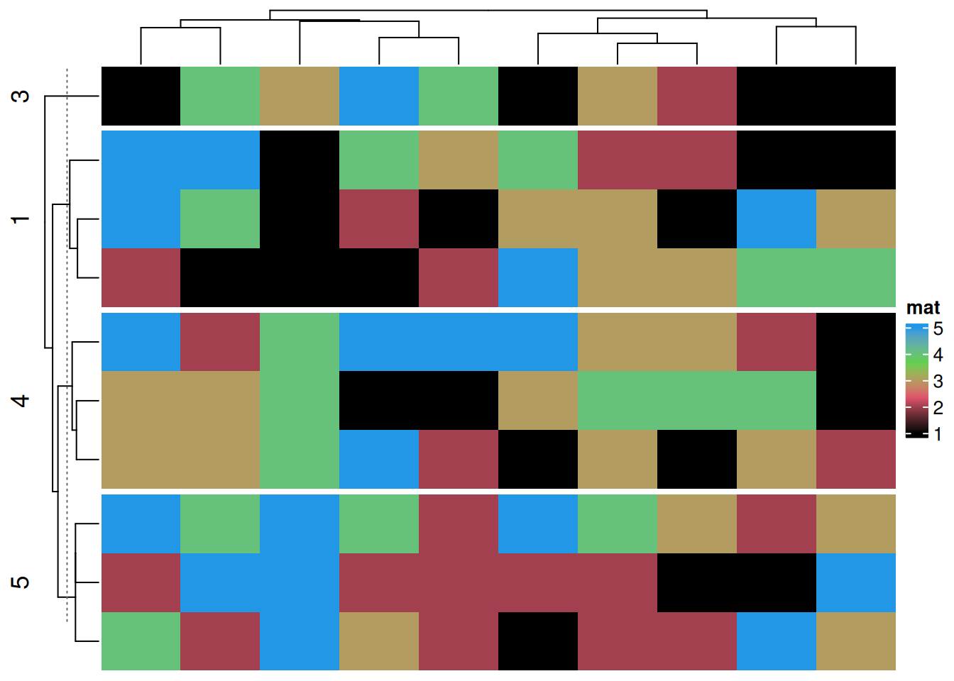
参数分割
可根据热图分割对标题,聚类参数等进行分割
# 参数分割
Heatmap(data_TCGA, name = "Methylation",
        row_km = 2,
        row_title_gp = gpar(col = c("#9A090A", "#0D4B99"), font = 1:2),
        row_names_gp = gpar(col = c("#748901", "#E6AC03"), fontsize = c(10, 12)),
        column_km = 3,
        column_title_gp = gpar(fill = c("#BFD641", "#FE9900", "#CC6CE7"), font = 1:3), #fill用于填充
        column_names_gp = gpar(col = c("#1D6103", "#E08804", "#5E0676"), fontsize = c(10, 12, 8)))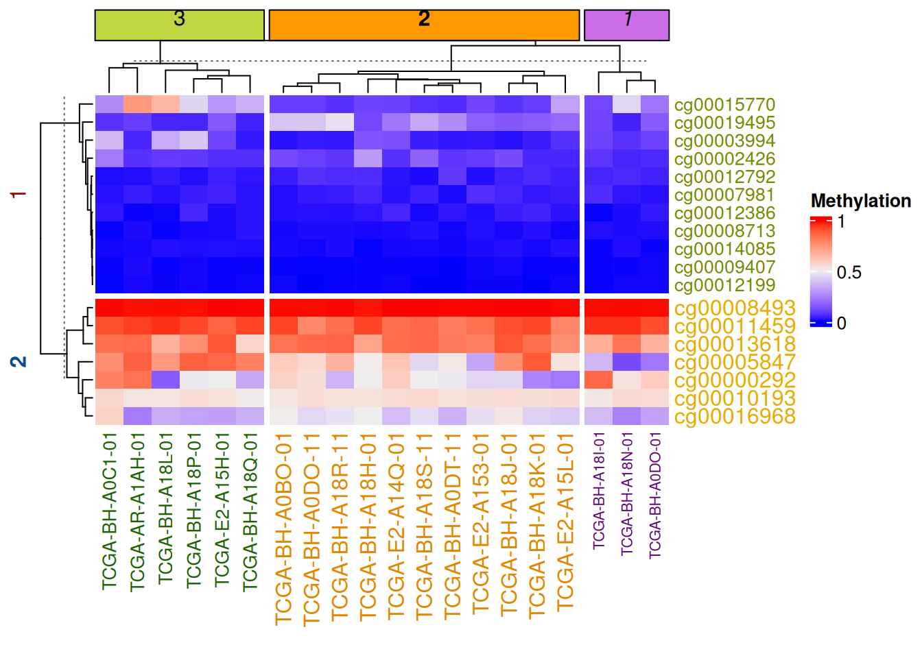
注释分割
可根据热图分割对边注释进行分割
# 注释分割
Heatmap(data_TCGA, name = "Methylation", row_km = 2, column_km = 3,
        top_annotation = HeatmapAnnotation(foo1 = 1:20, bar1 = anno_points(runif(20))),
        right_annotation = rowAnnotation(foo2 = 18:1, bar2 = anno_barplot(runif(18)))
)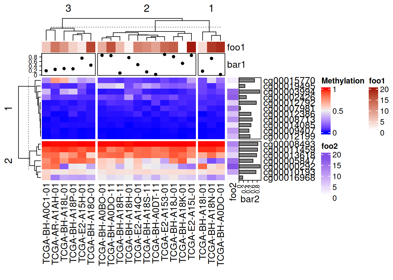
上图中添加的点图、热图、条图注释均随主热图分割
5. 标签添加
添加数据
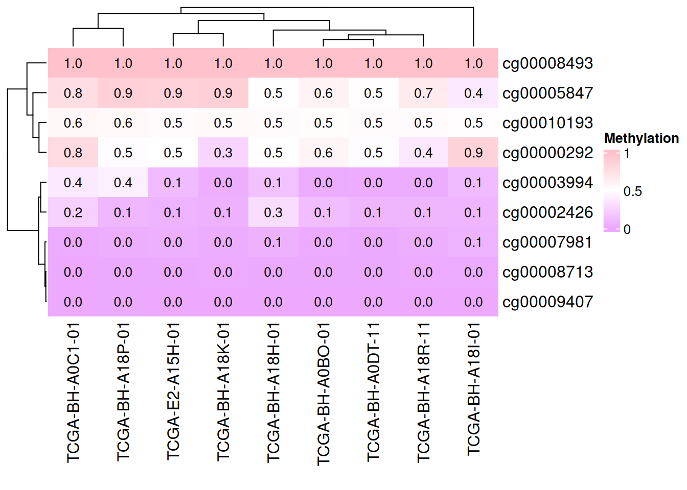
cell_fun 接受一个函数,该函数会被应用到热图的每个单元格上。函数的参数如下:
j: 列索引(列号)。i: 行索引(行号)。x,y: 单元格中心点的坐标(基于绘图设备的坐标系)。width,height: 单元格的宽度和高度。fill: 单元格对应的数值(即矩阵中的值)。
# 添加数据
small_mat = data_TCGA[1:9, 1:9]
col_fun = colorRamp2(c(0, 0.5, 1), c("#EBA7FE", "white", "pink"))
Heatmap(small_mat, name = "Methylation", col = col_fun,
        cell_fun = function(j, i, x, y, width, height, fill) {
          grid.text(sprintf("%.1f", small_mat[i, j]), x, y, gp = gpar(fontsize = 10))
        })
# 添加数据
small_mat = data_TCGA[1:9, 1:9]
Heatmap(small_mat, name = "Methylation",  col = col_fun,
        cell_fun = function(j, i, x, y, width, height, fill) {
          if(small_mat[i, j] > 0.5) #设定显示范围
            grid.text(sprintf("%.1f", small_mat[i, j]), x, y, gp = gpar(fontsize = 10)) #添加文本/数值
        })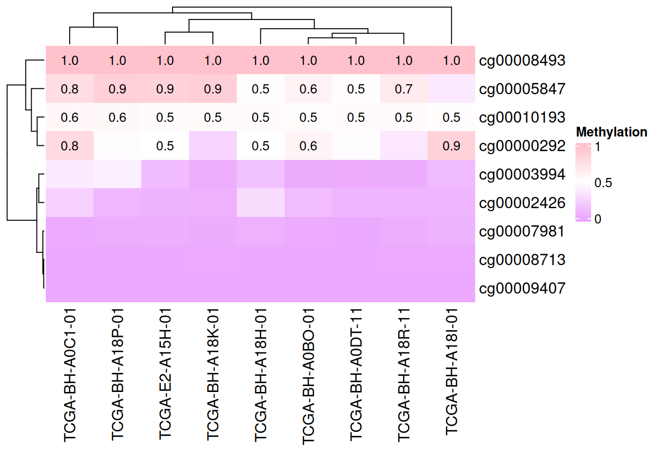
上图仅显示甲基化水平大于0.5的数据
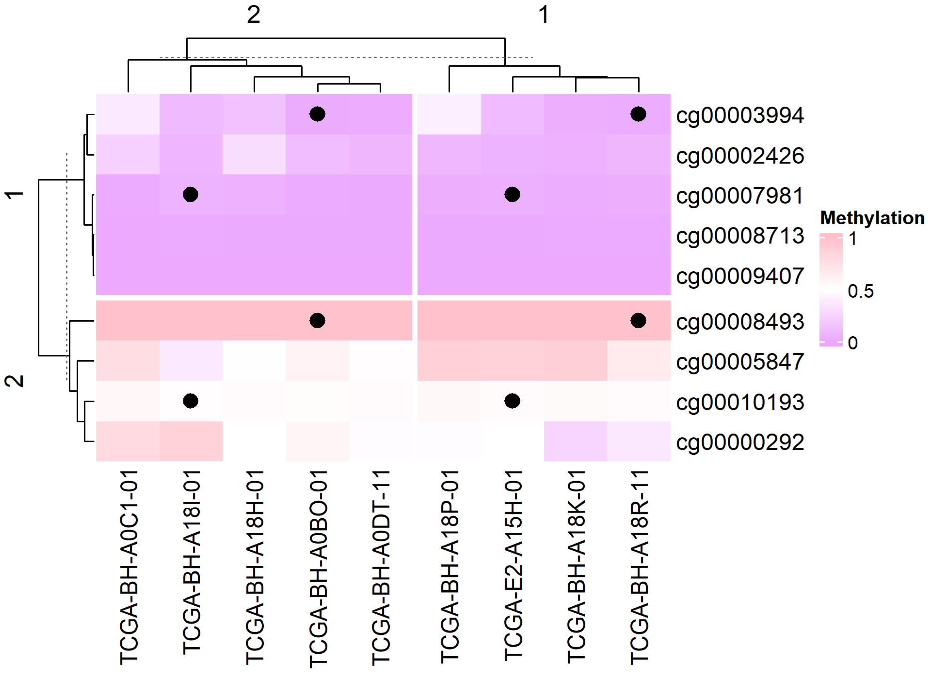
添加图形
# 添加图形
small_mat = data_TCGA[1:9, 1:9]
Heatmap(small_mat, name = "Methylation", col = col_fun,
        row_km = 2, column_km = 2,
        layer_fun = function(j, i, x, y, w, h, fill) {
          ind_mat = restore_matrix(j, i, x, y)
          ind = unique(c(ind_mat[1, 4], ind_mat[3, 2])) #定位,每个分割对应位置添加图形
          grid.points(x[ind], y[ind], pch = 16, size = unit(4, "mm")) #添加点
        }
)
6. 按相关系数排序的带注释热图
在生物标志物研究中 [4],列是按某个目标基因表达量排序的样本,行是与目标基因显著正/负相关的基因,顶部注释承载亚型/突变信息。关闭聚类后,目标基因的梯度(以及相关基因的楔形分布)一目了然——这就是无聚类的相关性热图。
set.seed(2026)
n_sam  <- 40
genes  <- paste0("Gene", sprintf("%03d", 1:299))
target <- rnorm(n_sam)                                   # 目标基因(类 TIM-3)表达量
subtype <- factor(sample(c("Classical", "Mesenchymal", "Neural", "Proneural"), n_sam, TRUE))
idh     <- factor(sample(c("WT", "Mutant"), n_sam, TRUE, prob = c(0.6, 0.4)))

mat <- matrix(rnorm(299 * n_sam), nrow = 299,
              dimnames = list(genes, paste0("S", seq_len(n_sam))))
# 模拟生物学:15 个基因与目标基因共变,10 个反向变化
pos_seed <- sample(genes, 15)
neg_seed <- sample(setdiff(genes, pos_seed), 10)
mat[pos_seed, ] <- mat[pos_seed, ] + outer(rep(1, 15), target) * 0.9
mat[neg_seed, ] <- mat[neg_seed, ] - outer(rep(1, 10), target) * 0.9
mat <- rbind(mat, "TARGET" = target)                     # 加入目标基因行

# 与目标基因相关的基因:正相关 top-15、负相关 top-10
cors      <- cor(t(mat[genes, ]), mat["TARGET", ])
pos_genes <- names(sort(cors[, 1], decreasing = TRUE))[1:15]
neg_genes <- names(sort(cors[, 1], decreasing = FALSE))[1:10]

sel  <- c(pos_genes, neg_genes)                          # 行:正相关块在前
mat_sel <- t(scale(t(mat[sel, ])))                       # 逐行 z-score
mat_sel[mat_sel >  3] <-  3
mat_sel[mat_sel < -3] <- -3
ord    <- order(mat["TARGET", ])                         # 列按目标基因排序
mat_sel <- mat_sel[, ord]

col_fun    <- circlize::colorRamp2(c(-3, 0, 3), c("#6699CC", "white", "#FF3C38"))
target_fun <- circlize::colorRamp2(c(-2, 0, 2), c("#2166ac", "white", "#b2182b"))

ha <- HeatmapAnnotation(
  `Target expression` = mat["TARGET", ord],
  Subtype = droplevels(subtype)[ord],
  IDH     = idh[ord],
  col = list(`Target expression` = target_fun,
             Subtype = c(Classical = "#CEDC7C", Mesenchymal = "#EA6767",
                         Neural = "#F7C07C", Proneural = "#445EAD"),
             IDH = c(WT = "#EA6767", Mutant = "#70C17A")))

Heatmap(mat_sel, name = "Z-score", top_annotation = ha,
        col = col_fun,
        cluster_rows = FALSE, cluster_columns = FALSE,   # 保留目标基因梯度
        row_split = factor(rep(c("Positively correlated", "Negatively correlated"),
                               c(length(pos_genes), length(neg_genes)))),
        border = TRUE)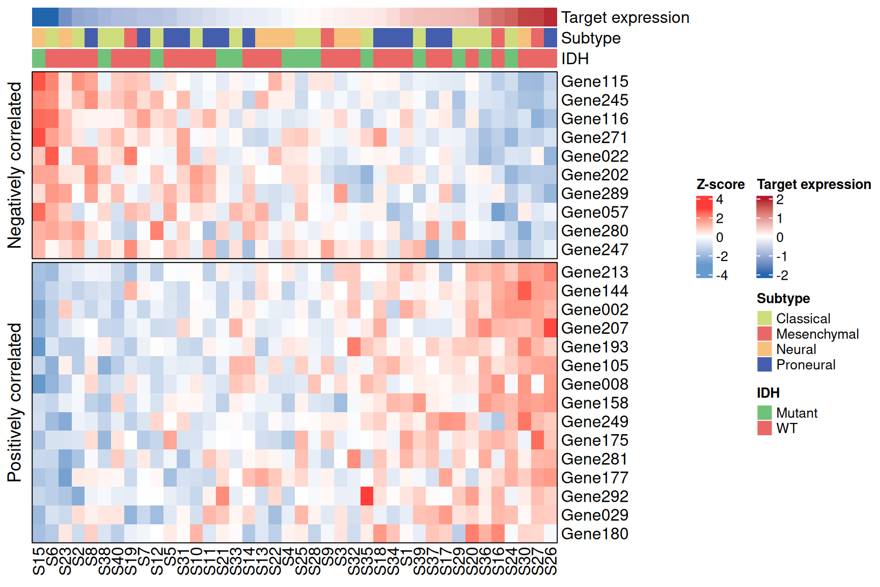
提示
实践要点
- 这里的行分割由分析结果驱动(相关系数的符号),而非聚类——
row_split接受任意因子。 - 绘图前先按目标基因对列排序,相关性强弱才会呈现为可见的楔形;务必保持
cluster_columns = FALSE,否则排序会被聚类破坏。 - 真实数据请用
cor.test()(Spearman)加 rho 与 P 值阈值来筛选相关基因,参考工作流如此实现。
应用场景
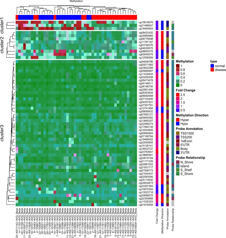
上图是基于 AVR 数据[1]中 59 个差异甲基化 ATG 位点的无监督层次聚类热图。红色表示 DNA 甲基化程度高,绿色表示甲基化程度低。
参考文献
[1] Radhakrishna U, Albayrak S, Alpay-Savasan Z, Zeb A, Turkoglu O, Sobolewski P, Bahado-Singh RO. Genome-Wide DNA Methylation Analysis and Epigenetic Variations Associated with Congenital Aortic Valve Stenosis (AVS). PLoS One. 2016 May 6;11(5):e0154010. doi: 10.1371/journal.pone.0154010. PMID: 27152866; PMCID: PMC4859473.
[2] Gu, Z. (2016) Complex heatmaps reveal patterns and correlations in multidimensional genomic data. Bioinformatics.Gu, Z. (2022) Complex Heatmap Visualization. iMeta.
[3] Tal Galili (2015). dendextend: an R package for visualizing, adjusting, and comparing trees of hierarchical clustering. Bioinformatics. DOI:10.1093/bioinformatics/btv428
[4] Wickham H, Vaughan D, Girlich M (2024). tidyr: Tidy Messy Data. R package version 1.3.1, CRAN: Package tidyr.
[5] Gu, Z. (2014) circlize implements and enhances circular visualization in R. Bioinformatics.
[6] Auguie B (2017). gridExtra: Miscellaneous Functions for “Grid” Graphics. R package version 2.3, CRAN: Package gridExtra.
[7] Kolde R (2019). pheatmap: Pretty Heatmaps. R package version 1.0.12, CRAN: Package pheatmap.
[8] Xiaofan Lu, et al. FigureYa: A Standardized Visualization Framework for Enhancing Biomedical Data Interpretation and Research Efficiency. iMetaMed. 2025. doi:10.1002/imm3.70005