import matplotlib.pyplot as plt
import numpy as np
import pandas as pd
import pingouin as pg
from statsmodels.graphics.agreement import mean_diff_plotBland-Altman 一致性图 (Python)
Bland-Altman 一致性图的 Python 对应版本——评估同一生理量的两种定量测量(参考方法 vs 床旁设备、可穿戴 vs 诊室血压)一致性的标准图形 [1]。每位受试者测量两次;图上以差值对均值作图,由均数之差(偏倚 bias)与 95% 一致性界限(bias ± 1.96 × 差值标准差)锚定解读。Pearson 相关很高并不等于一致:相关衡量线性关联,系统性偏高的方法同样相关得很好。
Python 有两个现成实现——pingouin.plot_blandaltman() [2] 与 statsmodels.graphics.agreement.mean_diff_plot() [3]——外加完全透明的 matplotlib 手工构造。本教程覆盖三条路线,以及针对比例偏倚的百分比差值变体。
本教程涵盖四种工作流:
-
pingouin.plot_blandaltman()(带置信区间); - 手绘 Bland-Altman 图(含偏倚的精确 CI);
-
statsmodels.mean_diff_plot()(Tukey 均值-差值图); - 针对异方差(比例偏倚)数据的百分比差值图。
Example
Setup
- 系统要求:跨平台(Linux/MacOS/Windows)
- 编程语言:Python
- 依赖包:
matplotlib、numpy、pandas、pingouin、statsmodels
Data Preparation
我们模拟与 R 版教程相同的方法比较研究:\(n = 120\) 份血清样本由参考方法与新的床旁方法(+6% 比例性高估、误差随浓度增大)测定。由此产生的喇叭形正是第 4 节要解决的问题。
rng = np.random.default_rng(2026)

n = 120
true_conc = rng.gamma(shape=2, scale=20, size=n)      # 右偏生物标志物
ref = true_conc * (1 + rng.normal(0, 0.05, n))        # 参考方法,约 5% CV
new = true_conc * (1 + rng.normal(0.06, 0.09, n))     # 新方法:+6% 偏倚,约 9% CV

avg = (ref + new) / 2      # 真值的最佳估计
diff = ref - new
methods = pd.DataFrame({"ref": ref, "new": new, "avg": avg, "diff": diff})
methods.head()| ref | new | avg | diff | |
|---|---|---|---|---|
| 0 | 18.048160 | 20.323912 | 19.186036 | -2.275753 |
| 1 | 4.758802 | 5.001305 | 4.880054 | -0.242503 |
| 2 | 58.156040 | 60.126686 | 59.141363 | -1.970646 |
| 3 | 24.333446 | 31.797007 | 28.065226 | -7.463561 |
| 4 | 27.793778 | 25.835174 | 26.814476 | 1.958604 |
Visualization
1. pingouin 一行代码
fig, ax = plt.subplots(figsize=(6.5, 4.8))
pg.plot_blandaltman(ref, new, ax=ax)
ax.set_title("pingouin.plot_blandaltman")
fig.tight_layout()
plt.show()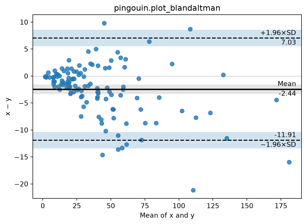
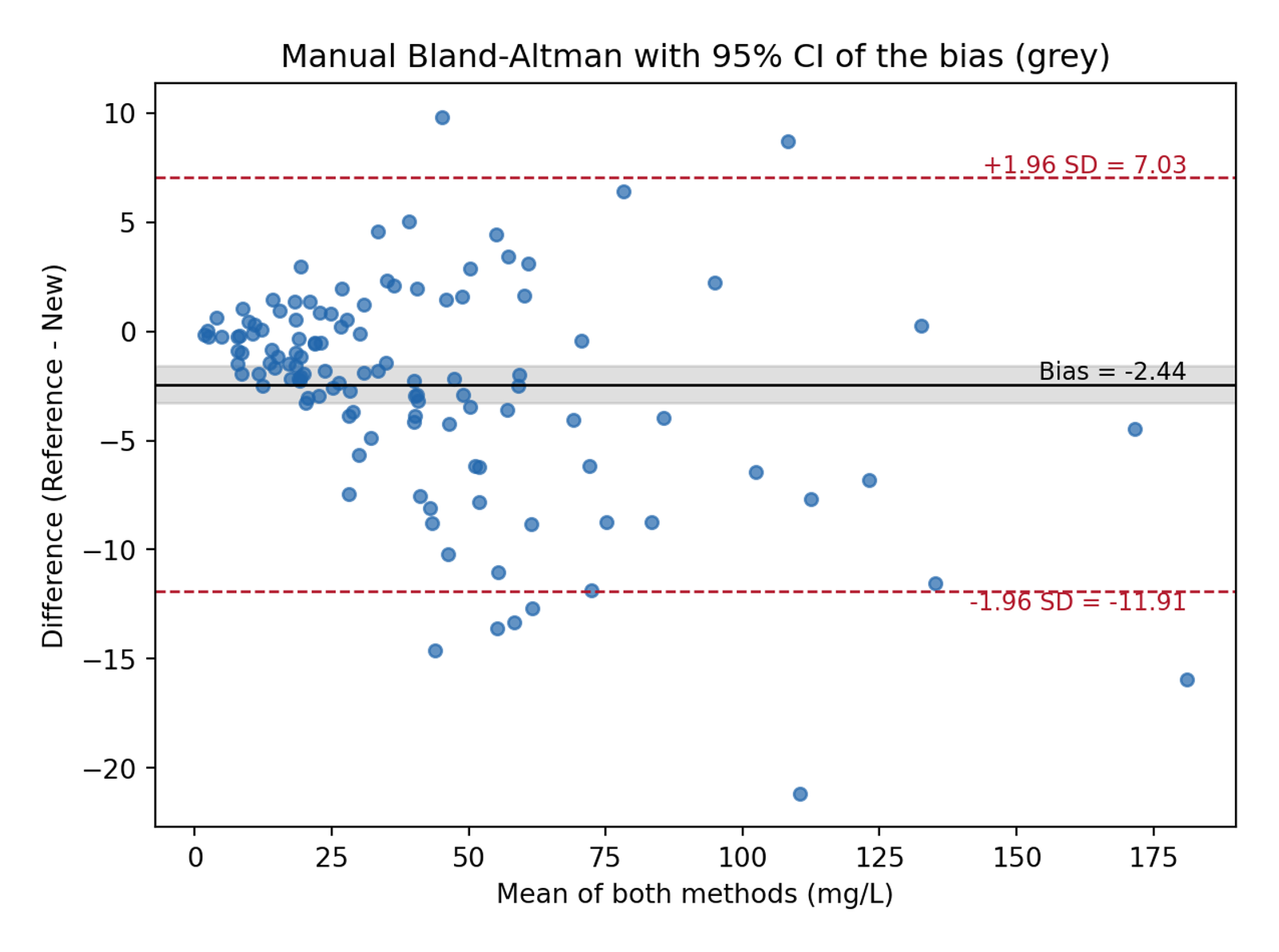
2. 手绘图:偏倚的精确置信区间
偏倚的置信区间用 \(\mathrm{SE} = s/\sqrt{n}\);一致性界限自身也有不确定性,\(\mathrm{SE}_{LoA} = \sqrt{s^2(1/n + 1.96^2/(2(n-1)))}\) [1]——小样本研究中必须报告。
bias, sd = diff.mean(), diff.std(ddof=1)
loa = (bias - 1.96 * sd, bias + 1.96 * sd)
se_bias = sd / np.sqrt(n)
se_loa = np.sqrt(sd**2 * (1 / n + 1.96**2 / (2 * (n - 1))))

fig, ax = plt.subplots(figsize=(6.5, 4.8))
ax.axhspan(bias - 1.96 * se_bias, bias + 1.96 * se_bias, color="grey", alpha=0.25)
ax.axhline(bias, color="black", lw=1)
ax.axhline(loa[0], color="#B2182B", ls="--", lw=1)
ax.axhline(loa[1], color="#B2182B", ls="--", lw=1)
ax.scatter(avg, diff, s=22, color="#2166AC", alpha=0.7)
ax.text(avg.max(), bias, f"  Bias = {bias:.2f}", va="bottom", ha="right", fontsize=9)
ax.text(avg.max(), loa[1], f"  +1.96 SD = {loa[1]:.2f}",
        va="bottom", ha="right", fontsize=9, color="#B2182B")
ax.text(avg.max(), loa[0], f"  -1.96 SD = {loa[0]:.2f}",
        va="top", ha="right", fontsize=9, color="#B2182B")
ax.set_xlabel("Mean of both methods (mg/L)")
ax.set_ylabel("Difference (Reference - New)")
ax.set_title("Manual Bland-Altman with 95% CI of the bias (grey)")
fig.tight_layout()
plt.show()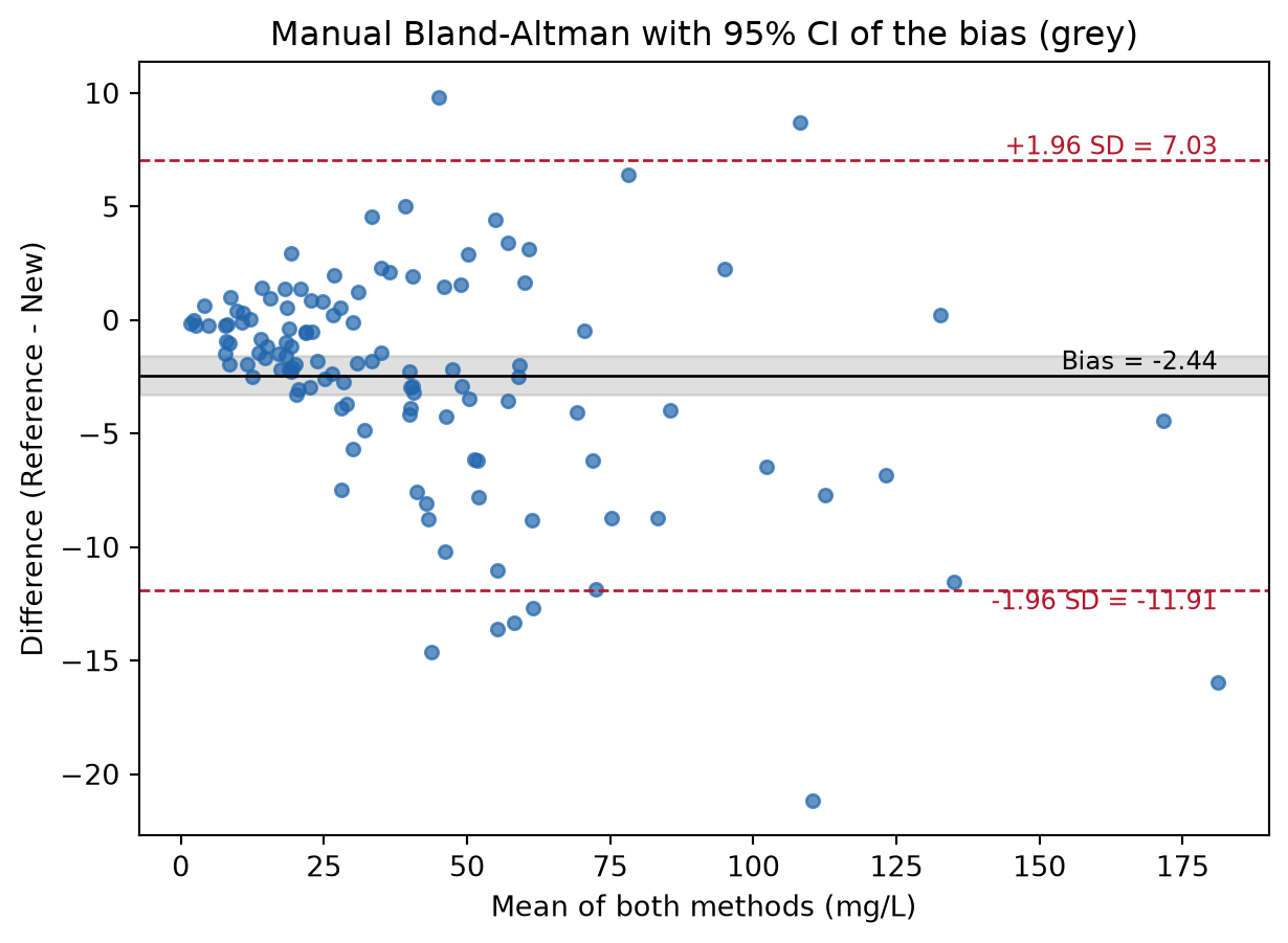
约 −2.4 mg/L 的平均差值即偏倚:新方法平均比参考方法读数偏高。一致性界限(±12 mg/L)是否可接受是结合判定阈值的临床判断,而非统计判断。
3. statsmodels 均值-差值图
fig, ax = plt.subplots(figsize=(6.5, 4.8))
mean_diff_plot(ref, new, ax=ax)
ax.set_title("statsmodels.graphics.agreement.mean_diff_plot")
fig.tight_layout()
plt.show()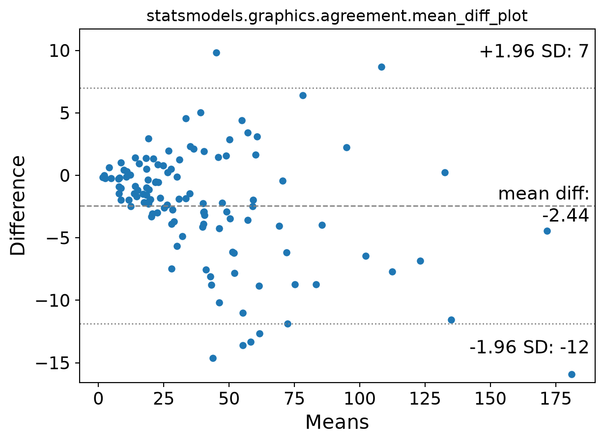
4. 针对比例偏倚的百分比差值图
第 1–3 节的喇叭形说明误差离散度随浓度增大。把差值表示为均值的百分比可恢复恒定离散度——一条偏倚、一对界限即可覆盖全量程——与对两次测量做对数变换等效。
pct = diff / avg * 100
pbias, psd = pct.mean(), pct.std(ddof=1)

fig, ax = plt.subplots(figsize=(6.5, 4.8))
ax.axhline(pbias, color="black", lw=1)
ax.axhline(pbias - 1.96 * psd, color="#B2182B", ls="--", lw=1)
ax.axhline(pbias + 1.96 * psd, color="#B2182B", ls="--", lw=1)
ax.scatter(avg, pct, s=22, color="#2166AC", alpha=0.7)
ax.set_xlabel("Mean of both methods (mg/L)")
ax.set_ylabel("Difference (% of mean)")
ax.set_title(f"Percentage difference (bias = {pbias:.1f}%)")
fig.tight_layout()
plt.show()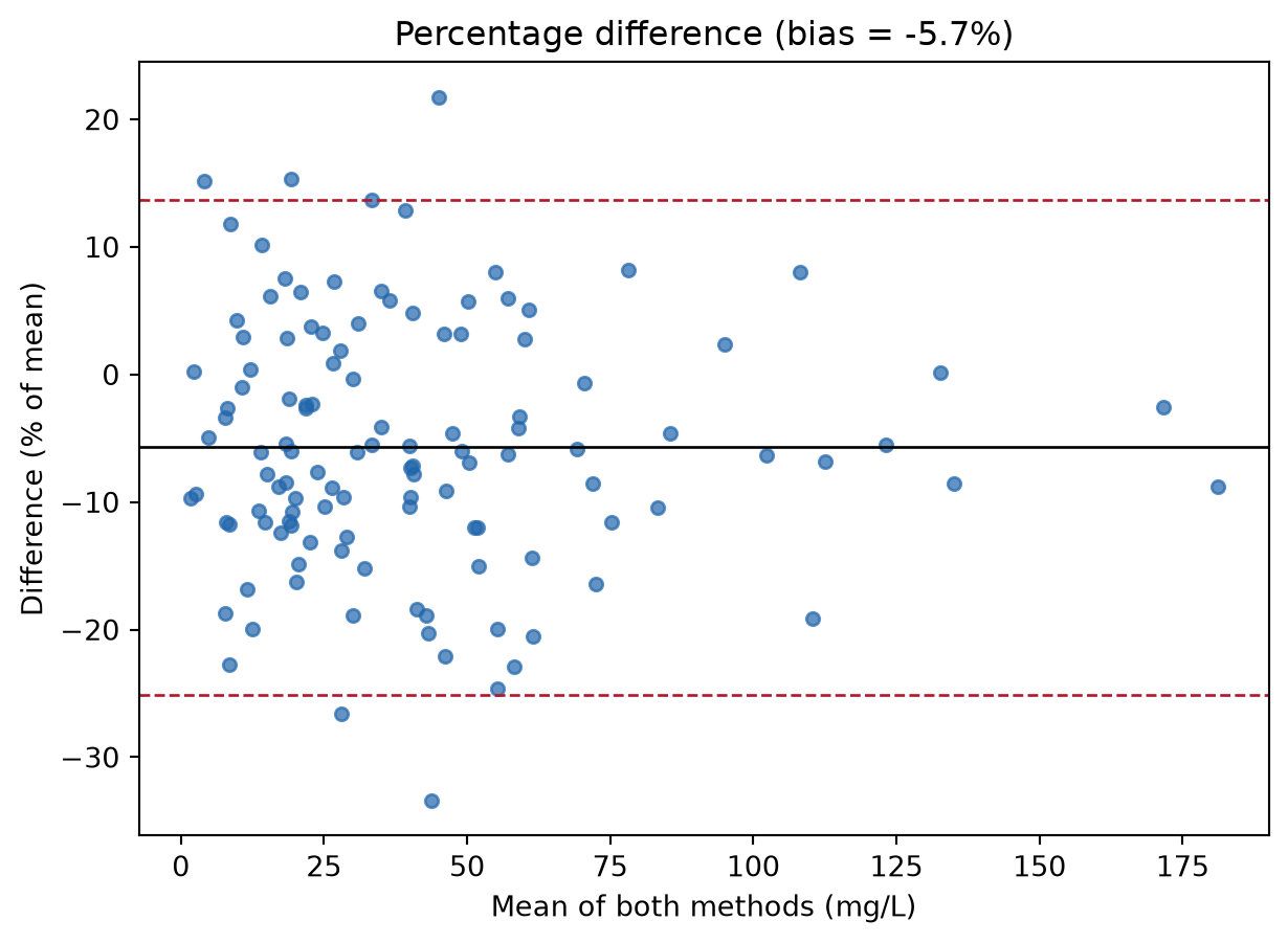
提示实践要点
- 差值对两方法的均值作图——对单一方法作图会在差值中引入虚假相关。
-
pingouin与statsmodels的默认标注不同;两者都不给出界限的置信区间——审稿人问到时用第 2 节的公式计算。 - 配对 t 检验不是一致性分析;报告图形加偏倚/界限,并在引用原始单位界限前检查喇叭形。
- 可复现性用
numpy.random.default_rng(seed)——旧式np.random.seed的全局状态在库之间不共享。
Application
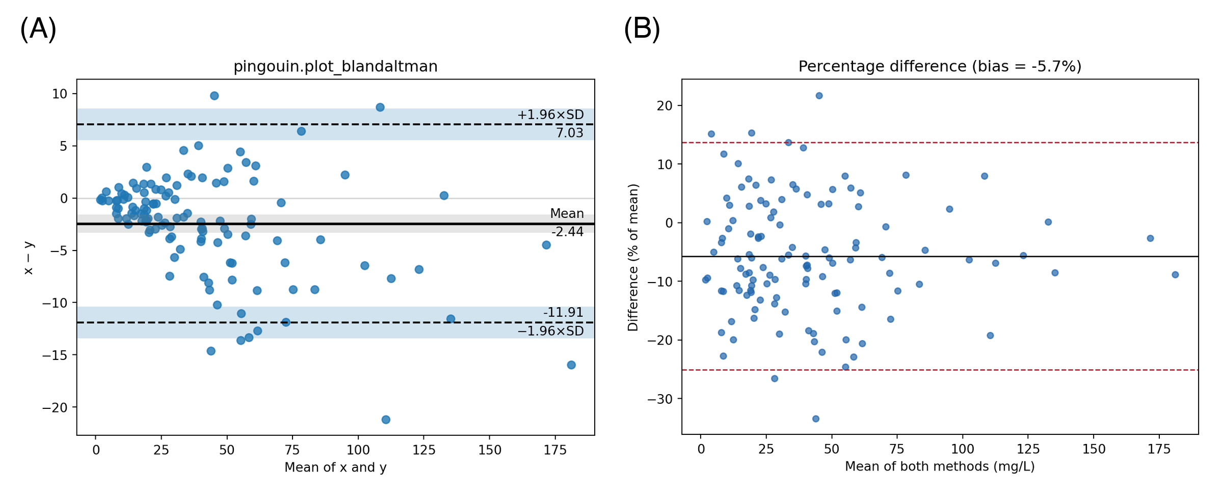
方法比较面板出现在实验室或临床更换仪器/设备的每一处:生化分析仪、床旁血糖/酮体仪、可穿戴与导管血压对比。下图模拟典型论文版式:(A) 带偏倚 CI 的手绘图与 (B) 处理比例偏倚的百分比变体。
Reference
[1] Bland JM, Altman DG. Measuring agreement in method comparison studies. Stat Methods Med Res. 1999;8(2):135-160. doi:10.1177/096228029900800204
[2] Vallat R. Pingouin: statistics in Python. J Open Source Softw. 2018;3(31):1026. doi:10.21105/joss.01026
[3] Seabold S, Perktold J. statsmodels: econometric and statistical modeling with Python. Proc 9th Python Sci Conf. 2010:92-96. doi:10.25080/Majora-92bf1922-011