# 安装包
if (!requireNamespace("data.table", quietly = TRUE)) {
  install.packages("data.table")
}
if (!requireNamespace("jsonlite", quietly = TRUE)) {
  install.packages("jsonlite")
}
if (!requireNamespace("ggrepel", quietly = TRUE)) {
  install.packages("ggrepel")
}
if (!requireNamespace("ggplot2", quietly = TRUE)) {
  install.packages("ggplot2")
}

# 加载包
library(data.table)
library(jsonlite)
library(ggrepel)
library(ggplot2)线性回归
注记
Hiplot 网站
本页面为 Hiplot Line Regression 插件的源码版本教程,您也可以使用 Hiplot 网站实现无代码绘图,更多信息请查看以下链接:
线性回归是一种对自变量和因变量之间关系进行线性建模的回归方法。只有一个自变量的情况称为简单回归,大于一个自变量情况的叫做多元回归。
环境配置
系统: Cross-platform (Linux/MacOS/Windows)
编程语言: R
依赖包:
data.table;jsonlite;ggrepel;ggplot2
sessioninfo::session_info("attached")─ Session info ───────────────────────────────────────────────────────────────
setting value
version R version 4.6.0 (2026-04-24)
os Ubuntu 24.04.4 LTS
system x86_64, linux-gnu
ui X11
language (EN)
collate C.UTF-8
ctype C.UTF-8
tz UTC
date 2026-05-09
pandoc 3.1.3 @ /usr/bin/ (via rmarkdown)
quarto 1.9.37 @ /usr/local/bin/quarto
─ Packages ───────────────────────────────────────────────────────────────────
package * version date (UTC) lib source
data.table * 1.18.4 2026-05-06 [1] RSPM
ggplot2 * 4.0.3.9000 2026-05-04 [1] Github (tidyverse/ggplot2@6870419)
ggrepel * 0.9.8 2026-03-17 [1] RSPM
jsonlite * 2.0.0 2025-03-27 [1] RSPM
[1] /home/runner/work/_temp/Library
[2] /opt/R/4.6.0/lib/R/site-library
[3] /opt/R/4.6.0/lib/R/library
* ── Packages attached to the search path.
──────────────────────────────────────────────────────────────────────────────数据准备
载入数据为自变量,因变量和分组。
# 加载数据
data <- data.table::fread(jsonlite::read_json("https://hiplot.cn/ui/basic/line-regression/data.json")$exampleData$textarea[[1]])
data <- as.data.frame(data)

# 整理数据格式
data$group <- factor(data$group, levels = unique(data$group))

# 查看数据
head(data)
value1 value2 group
1 36.8 29.44 G1
2 54.0 43.20 G1
3 26.0 26.00 G1
4 39.0 31.20 G1
5 33.0 29.70 G1
6 29.0 34.80 G1可视化
# 线性回归
## 定义方程
equation <- function(x, add_p = FALSE) {
  xs <- summary(x)
  lm_coef <- list(
    a = as.numeric(round(coef(x)[1], digits = 2)),
    b = as.numeric(round(coef(x)[2], digits = 2)),
    r2 = round(xs$r.squared, digits = 2),
    pval = xs$coef[2, 4]
  )
  if (add_p) {
    lm_eq <- substitute(italic(y) == a + b %.% italic(x) * "," ~ ~
  italic(R)^2 ~ "=" ~ r2 * "," ~ ~ italic(p) ~ "=" ~ pval, lm_coef)
  } else {
    lm_eq <- substitute(italic(y) == a + b %.% italic(x) * "," ~ ~
  italic(R)^2 ~ "=" ~ r2, lm_coef)
  }
  as.expression(lm_eq)
}
## 绘图
p <- ggplot(data, aes(x = value1, y = value2, colour = group)) +
  geom_point(show.legend = TRUE) +
  geom_smooth(method = "lm", se = T, show.legend = F) +
  geom_rug(sides = "bl", size = 1, show.legend = F) +
  scale_color_manual(values = c("#00468BFF","#ED0000FF")) +
  ggtitle("Line Reguression Plot") +
  theme_bw() +
  theme(text = element_text(family = "Arial"),
        plot.title = element_text(size = 12, hjust = 0.5),
        axis.title = element_text(size = 12),
        axis.text = element_text(size = 10),
        axis.text.x = element_text(angle = 0, hjust = 0.5,vjust = 1),
        legend.position = "right",
        legend.direction = "vertical",
        legend.title = element_text(size = 10),
        legend.text = element_text(size = 10))

## 使用 ggrepel 为每个组添加注释
repels <- rep("", nrow(data))
for (g in unique(data$group)) {
  fit <- lm(value2 ~ value1, data = data[data$group == g, ])
  v <- max(data[data$group == g, "value2"])
  repels[which(data$value2 == v)[1]] <- equation(fit, add_p = F)
}
p <- p + geom_text_repel(
  data = data,
  label = repels,
  size = 4,
  force = 5,
  label.padding = 5,
  na.rm = TRUE,
  min.segment.length = 100,
  show.legend = FALSE,
  nudge_x = 0,
  nudge_y = 0
  )

p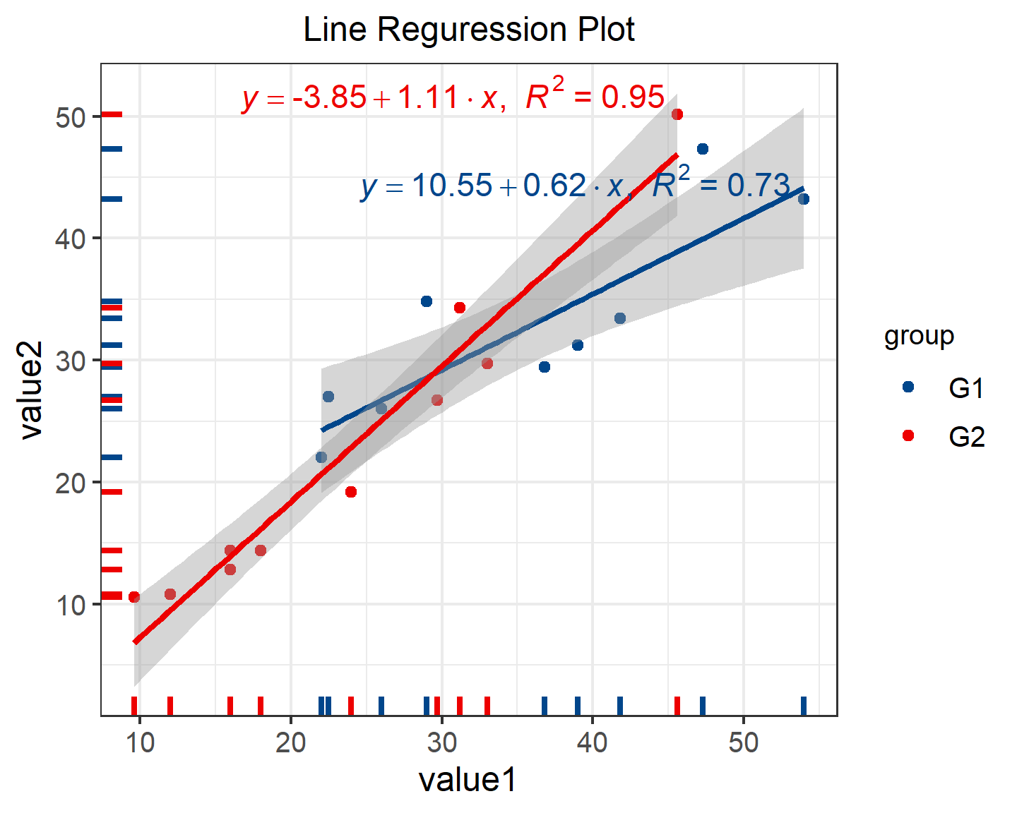
不同颜色表示不同分组,可添加线性回归方程,R的平方越接近 1,说明拟合的曲线和实际曲线越趋近。灰色条带代表 95% 置信区间。