# 安装必要的包
if (!requireNamespace("pROC", quietly = TRUE)) {
  install.packages("pROC")
}
if (!requireNamespace("plotROC", quietly = TRUE)) {
  install.packages("plotROC")
}
if (!requireNamespace("timeROC", quietly = TRUE)) {
  install.packages("timeROC")
}

# 加载包
library(survival)
library(dplyr)
library(ggplot2)
library(pROC)
library(plotROC)
library(timeROC)ROC 曲线
受试者工作特征(Receiver Operating Characteristic,ROC)曲线用于评估二元分类器——最常见的是临床预测模型——在所有可能决策阈值下的区分能力(discrimination)。它以灵敏度(真阳性率)对 1 − 特异度(假阳性率)作图,并用曲线下面积(AUC)概括:0.5 表示区分能力不优于随机猜测,1.0 表示完美区分。在临床研究中,ROC 分析是报告诊断与预后模型性能的标准工具之一,通常与校准曲线、决策曲线分析配合使用(见配套教程)。
本教程涵盖 R 中四种实用的 ROC 工作流:
- 基础 ROC 曲线及 AUC 与 bootstrap 置信区间(
pROC); - 使用 DeLong 检验比较两个模型的区分能力(
pROC); - 自动报告 AUC 的发表级 ROC 曲线(
plotROC); - 生存结局在固定时间点的 Time-dependent ROC(
timeROC)。
示例
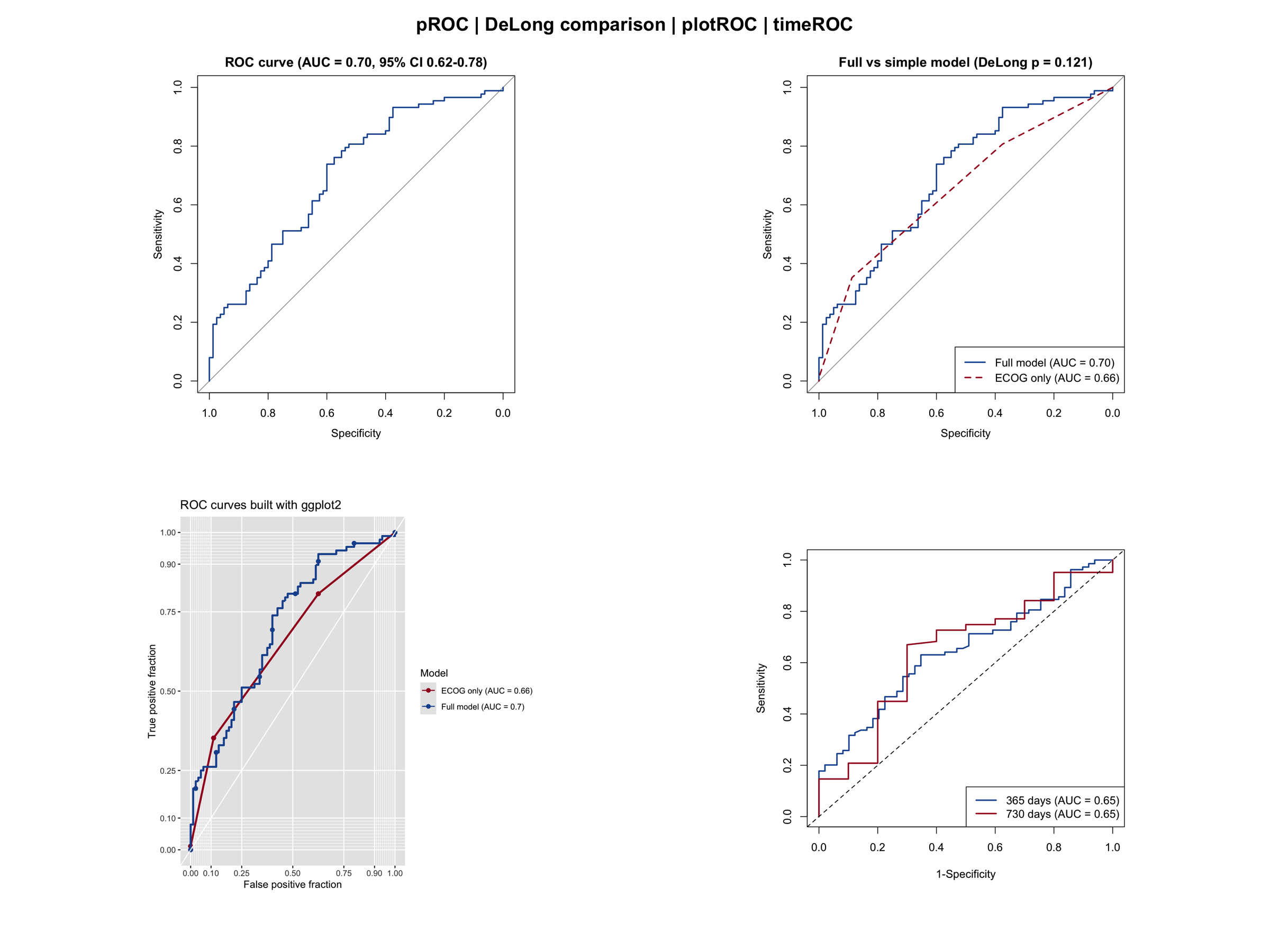
环境配置
系统要求:跨平台(Linux/MacOS/Windows)
编程语言:R
依赖包:
survival;dplyr;pROC;plotROC;timeROC;ggplot2
sessioninfo::session_info("attached")─ Session info ───────────────────────────────────────────────────────────────
setting value
version R version 4.6.1 (2026-06-24)
os Ubuntu 24.04.5 LTS
system x86_64, linux-gnu
ui X11
language (EN)
collate C.UTF-8
ctype C.UTF-8
tz UTC
date 2026-10-29
pandoc 3.1.3 @ /usr/bin/ (via rmarkdown)
quarto 1.10.19 @ /usr/local/bin/quarto
─ Packages ───────────────────────────────────────────────────────────────────
! package * version date (UTC) lib source
P dplyr * 1.2.1 2026-04-03 [?] RSPM
P ggplot2 * 4.0.3.9000 2026-10-26 [?] Github (tidyverse/ggplot2@b638d65)
P plotROC * 2.3.3 2025-08-25 [?] RSPM
P pROC * 1.19.1 2026-08-27 [?] RSPM
survival * 3.8-6 2026-01-16 [3] CRAN (R 4.6.1)
timeROC * 0.4.1 2026-04-10 [1] RSPM
[1] /home/runner/.cache/R/renv/library/Bizard-5140bdc6/linux-ubuntu-noble/R-4.6/x86_64-pc-linux-gnu
[2] /home/runner/work/_temp/Library
[3] /opt/R/4.6.1/lib/R/library
* ── Packages attached to the search path.
P ── Loaded and on-disk path mismatch.
──────────────────────────────────────────────────────────────────────────────数据准备
我们使用 survival 包内置的 lung 数据集(北中部癌症治疗组肺癌临床试验)[1]。定义一个二元终点——随访第一年内死亡——并拟合两个 logistic 模型:一个使用五个协变量的完整模型,一个仅使用 ECOG 体能评分的简单模型。同时构建 Cox 模型得到连续型风险评分,用于 Time-dependent ROC 分析。
# lung 数据集内置于 survival 包
data(lung, package = "survival")

lung2 <- lung %>%
  filter(complete.cases(age, sex, ph.ecog, ph.karno, pat.karno, meal.cal, wt.loss)) %>%
  mutate(y1y = as.integer(time < 365 & status == 2))  # 365 天内死亡
  # 注意:365 天内删失的患者在此被计为非事件;实际分析中建议仅纳入随访
  # 满 365 天的患者,或使用删失感知的方法(见下文 time-dependent ROC)。

cat("样本量:", nrow(lung2), " 1年死亡数:", sum(lung2$y1y), "\n")
样本量: 168 1年死亡数: 88 # 两个用于 1 年死亡率的 logistic 模型
m_full <- glm(y1y ~ age + sex + ph.ecog + meal.cal + wt.loss,
data = lung2, family = binomial)
m_simple <- glm(y1y ~ ph.ecog, data = lung2, family = binomial)
# 由 Cox 模型得到连续型风险评分(用于 time-dependent ROC)
cph0 <- coxph(Surv(time, status) ~ age + sex + ph.ecog + wt.loss, data = lung2)
lung2$risk_score <- as.numeric(predict(cph0, type = "risk"))
# 将每个模型的预测概率存为列(melt_roc 需要)
lung2$risk_full <- fitted(m_full)
lung2$risk_ecog <- fitted(m_simple)可视化
1. 基础 ROC 曲线与 AUC 置信区间
roc_full <- roc(lung2$y1y, fitted(m_full), quiet = TRUE)
set.seed(2026)  # 固定随机种子,保证 bootstrap 置信区间跨渲染可复现
ci_full  <- ci.auc(roc_full, method = "bootstrap", boot.n = 1000)

plot(roc_full, col = "#2166AC", lwd = 2,
     main = sprintf("ROC curve (AUC = %.2f, 95%% CI %.2f-%.2f)",
                    as.numeric(auc(roc_full)),
                    ci_full[1], ci_full[3]))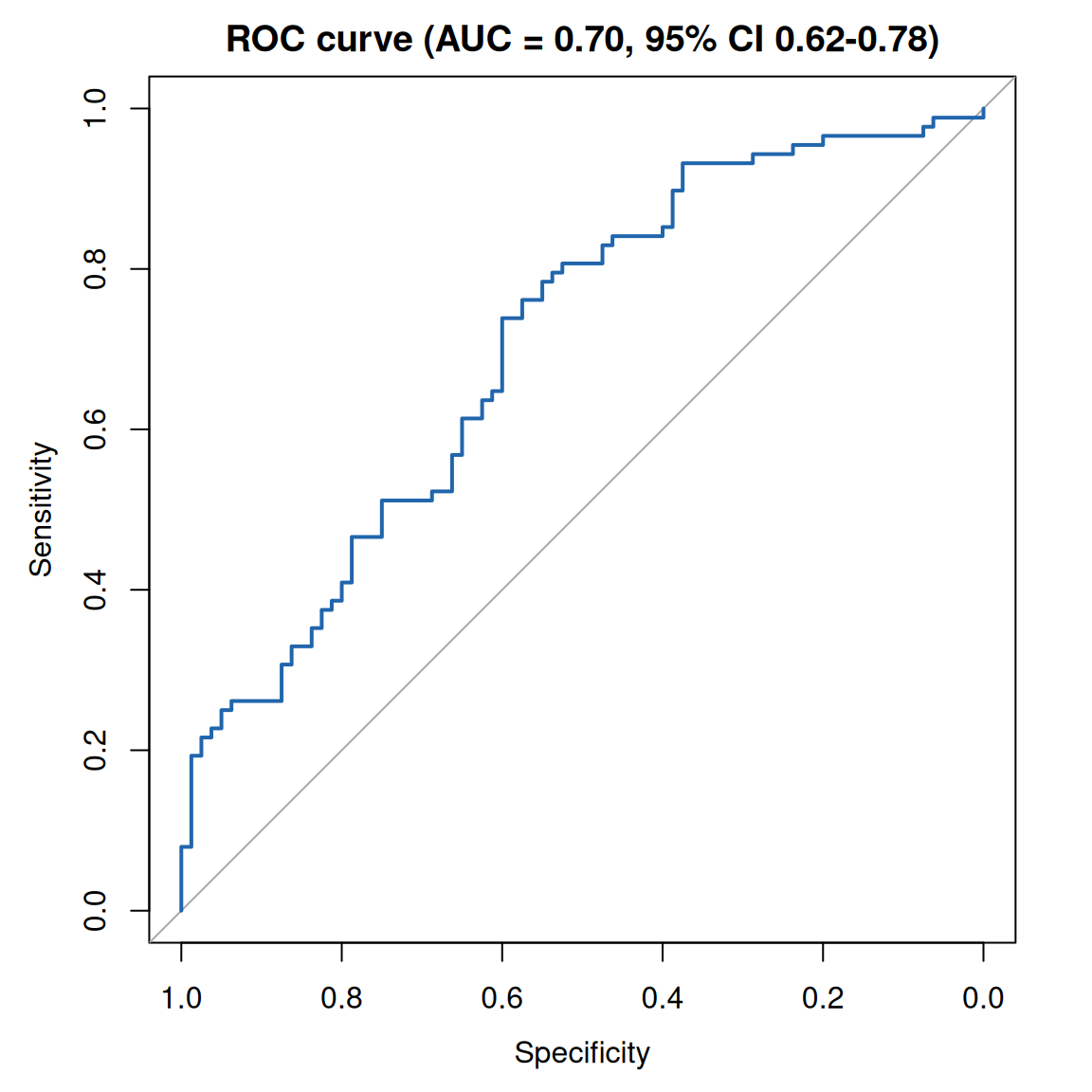
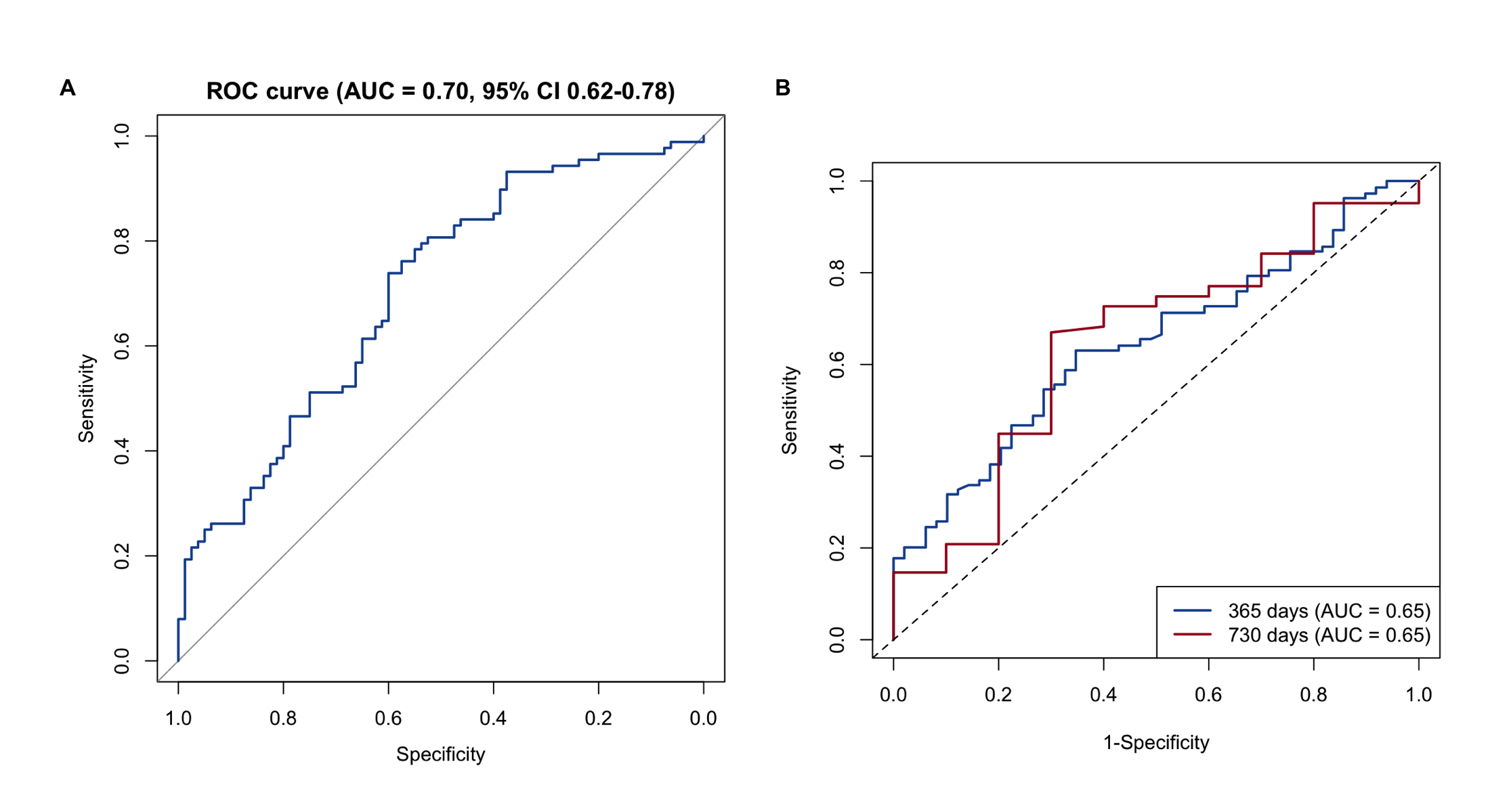
AUC 为 0.70 表示模型对 1 年死亡具有可接受的区分能力。bootstrap 置信区间量化了该估计的抽样不确定性。
2. 使用 DeLong 检验比较两个模型
常见的问题是:完整模型的额外协变量是否真的比简单模型提升了区分能力?DeLong 检验无需重抽样即可比较配对的 ROC 曲线。
roc_simple <- roc(lung2$y1y, fitted(m_simple), quiet = TRUE)
roc_test <- roc.test(roc_full, roc_simple, method = "delong")

plot(roc_full, col = "#2166AC", lwd = 2,
     main = sprintf("Full vs simple model (DeLong p = %.3f)", roc_test$p.value))
plot(roc_simple, col = "#B2182B", lwd = 2, lty = 2, add = TRUE)
legend("bottomright",
       legend = c(sprintf("Full model (AUC = %.2f)", auc(roc_full)),
                  sprintf("ECOG only (AUC = %.2f)", auc(roc_simple))),
       col = c("#2166AC", "#B2182B"), lwd = 2, lty = c(1, 2))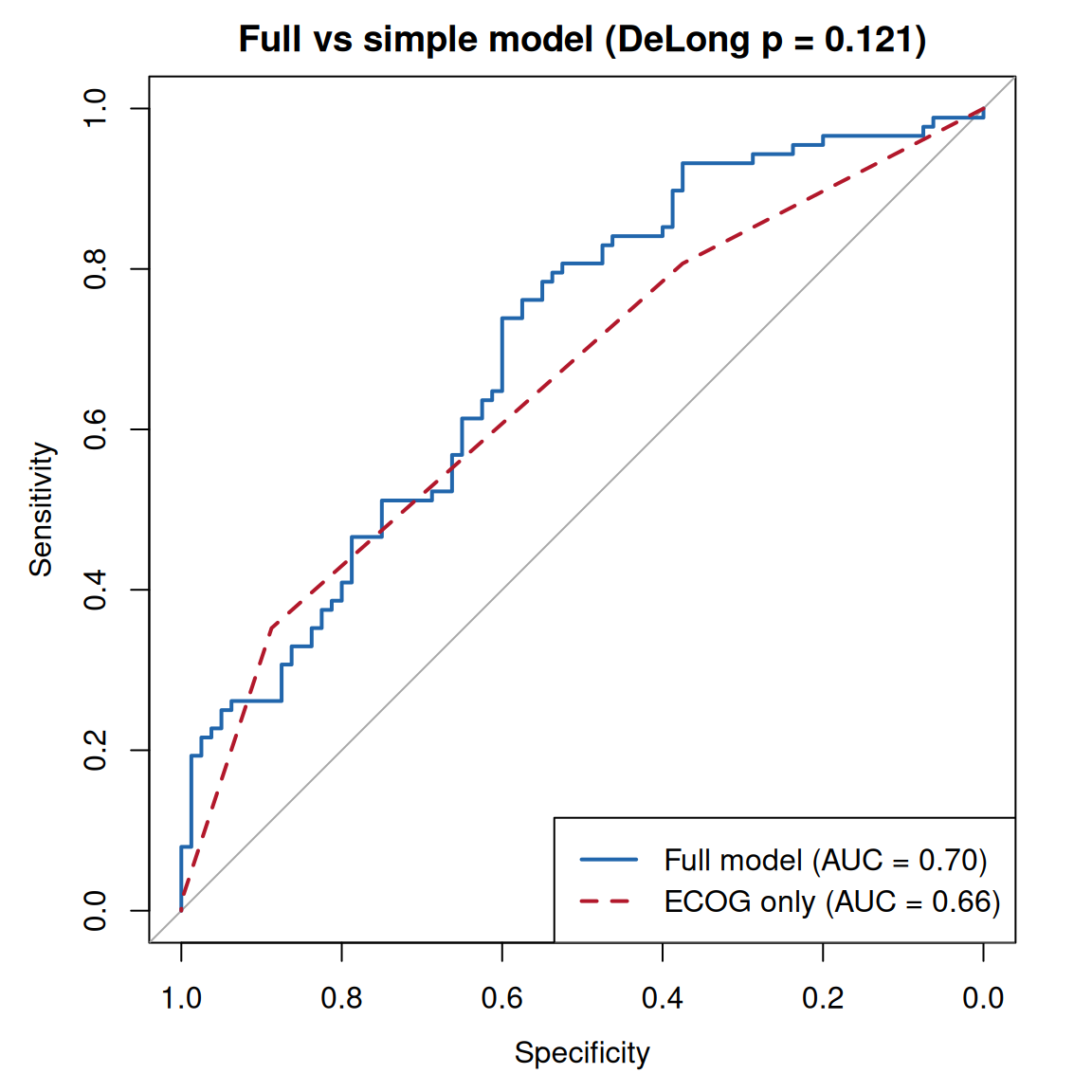
本例中差异不显著(p = 0.121),提示在这个小样本数据中不宜宣称额外协变量带来了增益。
3. 最佳截断值选择
best <- coords(roc_full, x = "best", input = "threshold",
               best.method = "youden", ret = c("threshold", "specificity", "sensitivity"))
print(best)
threshold specificity sensitivity
1 0.4555072 0.6 0.7386364plot(roc_full, col = "#2166AC", lwd = 2, print.thres = "best",
print.thres.best.method = "youden",
main = "ROC curve with Youden-optimal threshold")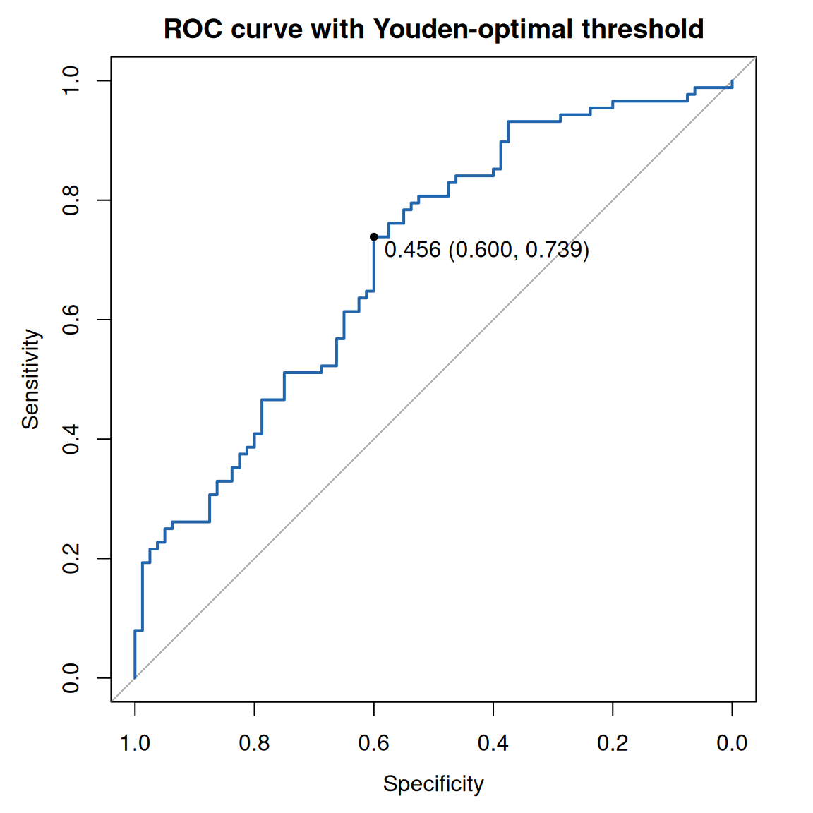
Youden 指数选取使灵敏度 + 特异度 − 1 最大化的阈值。注意“最佳”截断值依赖于具体场景:应结合临床代价(假阳性与假阴性的危害)来选择,例如借助决策曲线分析。
4. 使用 plotROC 绘制发表级 ROC 曲线
longdf <- melt_roc(lung2, d = "y1y", m = c("risk_full", "risk_ecog")) |>
  mutate(name = ifelse(name == "risk_full", "Full model", "ECOG only"))

# 命名向量:无论水平顺序如何都能正确匹配颜色与标签
model_colors <- c("Full model" = "#2166AC", "ECOG only" = "#B2182B")
model_labels <- c("Full model" = paste0("Full model (AUC = ", round(auc(roc_full), 2), ")"),
                  "ECOG only"  = paste0("ECOG only (AUC = ", round(auc(roc_simple), 2), ")"))
ggplot(longdf, aes(d = D, m = M, color = name)) +
  geom_roc(labels = FALSE, linewidth = 1) +
  style_roc(theme = theme_grey()) +
  scale_color_manual(values = model_colors, labels = model_labels, name = "Model") +
  labs(title = "ROC curves built with ggplot2")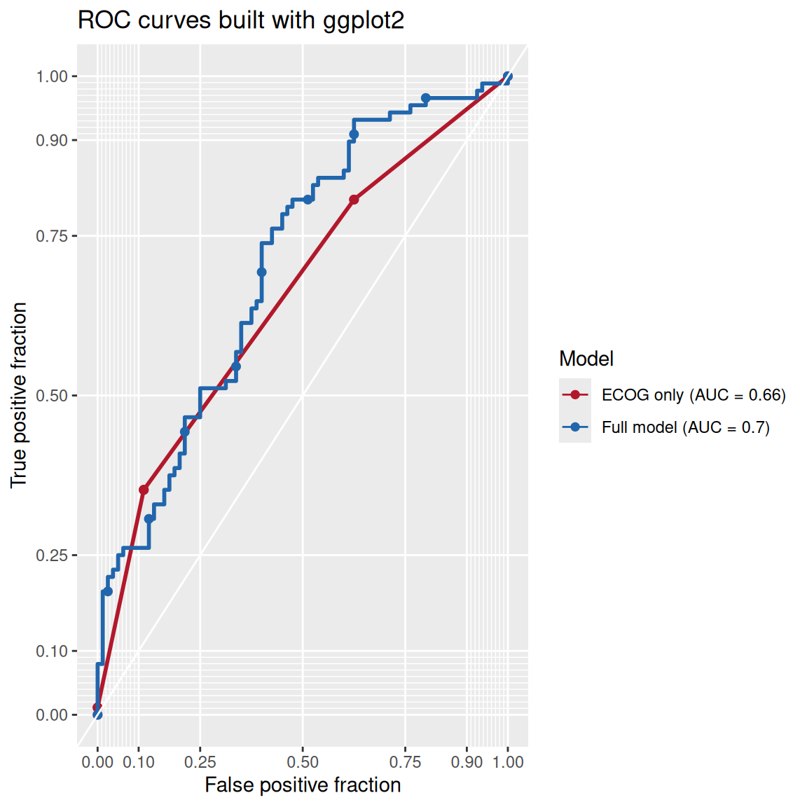
melt_roc() 将数据转换为长格式,geom_roc() 绘制曲线;AUC 由 pROC 计算并在图例中显示。
5. 使用 timeROC 的 Time-dependent ROC
对于生存终点,标准 ROC 无法处理删失。Time-dependent ROC 评估固定时间点的区分能力,例如用 Cox 风险评分预测 1 年和 2 年死亡率 [3]。
tr <- timeROC(T = as.numeric(lung2$time),
              delta = ifelse(lung2$status == 2, 1, 0),  # 1 = 事件, 0 = 删失
              marker = lung2$risk_score, cause = 1,
              weighting = "marginal",
              times = c(365, 730), ROC = TRUE, iid = TRUE)

plot(tr, time = 365, col = "#2166AC", lwd = 2,
     title = "Time-dependent ROC of the Cox risk score")
plot(tr, time = 730, col = "#B2182B", lwd = 2, add = TRUE)
legend("bottomright",
       legend = sprintf("%d days (AUC = %.2f)", c(365, 730), tr$AUC),
       col = c("#2166AC", "#B2182B"), lwd = 2)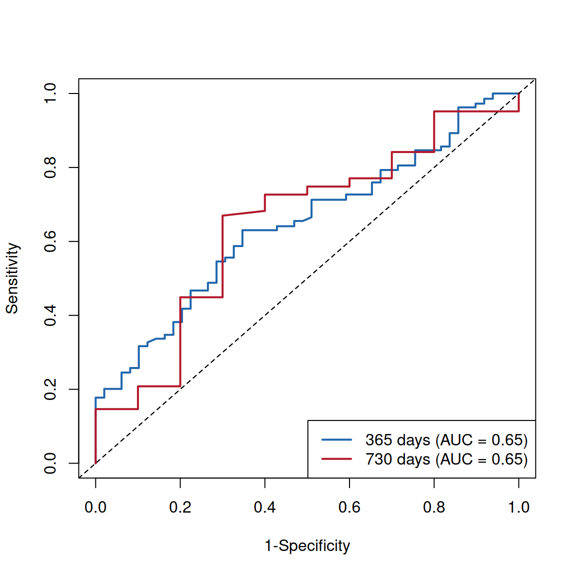
关键细节:delta 使用 0 = 删失、1 = 感兴趣事件的编码(注意这不是 lung 数据中 status 的原始编码——那里 1 表示删失);风险评分是由 Cox 模型导出的连续型 marker。由于设置了 iid = TRUE,可以通过 confint(tr) 获得 time-dependent AUC 的置信区间。
应用
Time-dependent ROC 曲线广泛用于肿瘤预后模型论文中,以报告在临床有意义的时间点(1、3、5 年)的区分能力,常与校准曲线、决策曲线分析并列出现。下图按照论文常用版式组装本教程的输出:(A) 二元模型的标准 ROC;(B) 固定时间点的 time-dependent ROC。
参考文献
[1] Loprinzi CL, Laurie JA, Wieand HS, et al. Prospective evaluation of prognostic variables from patient-completed questionnaires. North Central Cancer Treatment Group. J Clin Oncol. 1994;12(3):601-607. doi:10.1200/JCO.1994.12.3.601
[2] Robin X, Turck N, Hainard A, et al. pROC: an open-source package for R and S+ to analyze and compare ROC curves. BMC Bioinformatics. 2011;12:77. doi:10.1186/1471-2105-12-77
[3] Blanche P, Dartigues JF, Jacqmin-Gadda H. Estimating and comparing time-dependent areas under receiver operating characteristic curves for censored event times with competing risks. Stat Med. 2013;32(30):5381-5397. doi:10.1002/sim.5958
[4] Sachs MC. plotROC: A Tool for Plotting ROC Curves. J Stat Softw Code Snippets. 2017;79(2):1-12. doi:10.18637/jss.v079.c02