箱线图（Python）

🤖 AI Skill — Download the Bizard unified skill for your AI assistant ⬇️ Download Skill ZIP

🔌 MCP Server — Let AI agents (Claude Code, Cursor, …) query Bizard live: claude mcp add bizard -- npx @openbiox/bizard-mcp — or the free hosted instance (no install, faster from mainland China): claude mcp add --transport http bizard http://biotree.top:38123/bizard-mcp/mcp 📖 MCP Docs

📖 Cite Bizard — if Bizard helps your research, please cite: Li, K., Zheng, H., Huang, K., et al. (2026). Bizard: A Community-Driven Platform for Accelerating and Enhancing Biomedical Data Visualization. iMetaMed, e70038. 🔗 DOI / BibTeX

箱线图通过中位数、四分位数和离群值概括数值型变量的分布。在生物医学研究中，箱线图是比较不同基因型、批次或处理组之间生物标志物水平的标准紧凑展示方式。Python 的 seaborn 构建在 matplotlib 之上，提供缺口（notch）、分组和散点叠加等多种出版级变体。

示例

环境配置

• 系统要求：跨平台（Linux/MacOS/Windows）
• 编程语言：Python
• 依赖包：matplotlib、seaborn、pandas、numpy

import matplotlib.pyplot as plt
import seaborn as sns
import pandas as pd
import numpy as np

数据准备

我们模拟三种基因型（WT、HET、KO）的血清生物标志物检测数据，并为分组变体加入性别因素；每个基因型 60 个重复以保证四分位数估计的稳定性。

np.random.seed(7)

genotypes = ['WT', 'HET', 'KO']
n_per_genotype = 60
df = pd.DataFrame({
    'Genotype': np.repeat(genotypes, n_per_genotype),
    'Sex': np.tile(np.repeat(['Female', 'Male'], n_per_genotype // 2), 3),
    'Biomarker': np.concatenate([
        np.random.lognormal(1.2, 0.45, n_per_genotype),
        np.random.lognormal(1.55, 0.45, n_per_genotype),
        np.random.lognormal(1.95, 0.55, n_per_genotype),
    ])
})
# 在 KO 组注入若干极端值，用于演示离群值展示
df.loc[df.index[-3:], 'Biomarker'] *= 3.5

可视化

基础箱线图

箱体跨越四分位距（IQR），中线为中位数，须线延伸至 1.5 × IQR；超出该范围的点以离群值（fliers）绘制。

plt.figure(figsize=(5.5, 4.2))
ax = sns.boxplot(data=df, x='Genotype', y='Biomarker',
                 color='#8da0cb', width=0.5, linewidth=1.0,
                 fliersize=3, flierprops=dict(markerfacecolor='0.4'))
ax.set_xlabel('Genotype')
ax.set_ylabel('Biomarker level (ng/mL)')
ax.spines[['top', 'right']].set_visible(False)
plt.tight_layout()
plt.show()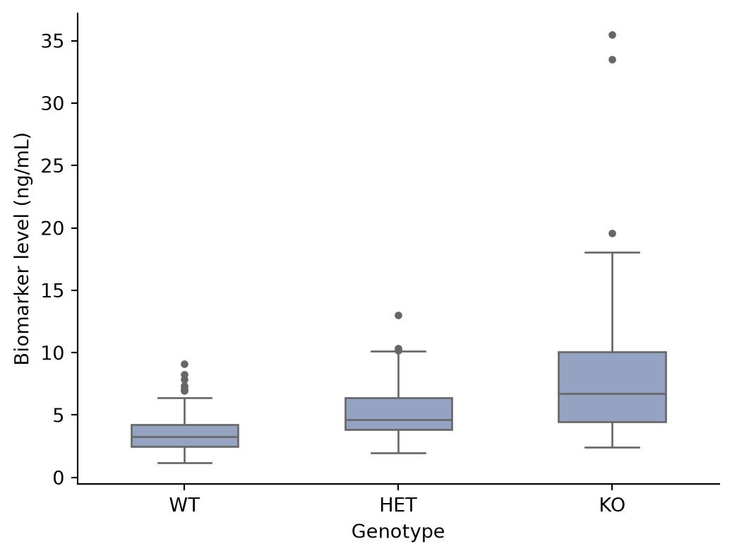

图 1: 不同基因型血清生物标志物的箱线图

箱线图叠加散点

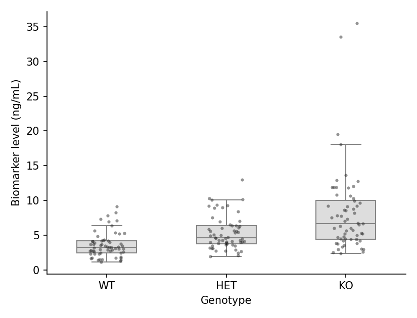
由于箱体会隐藏原始数据，叠加单个观测值是出版界推荐的风格：设置 showfliers=False 并添加一层 stripplot。

plt.figure(figsize=(5.5, 4.2))
ax = sns.boxplot(data=df, x='Genotype', y='Biomarker',
                 color='#dddddd', width=0.5, linewidth=1.0,
                 showfliers=False)
sns.stripplot(data=df, x='Genotype', y='Biomarker',
              color='#2b2b2b', size=3, alpha=0.5, jitter=0.15, ax=ax)
ax.set_xlabel('Genotype')
ax.set_ylabel('Biomarker level (ng/mL)')
ax.spines[['top', 'right']].set_visible(False)
plt.tight_layout()
plt.show()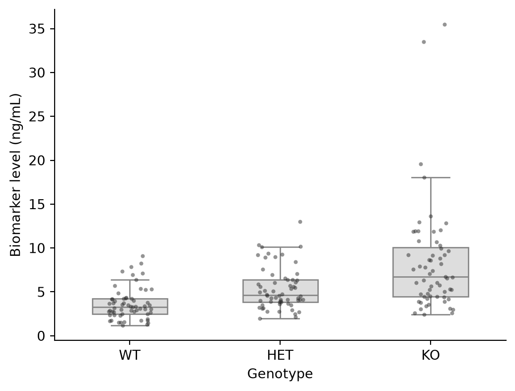

图 2: 箱线图叠加原始数据点

分组箱线图

第二个因素映射到 hue，在每个类别内生成成对的箱体——典型的配对或双队列比较形式。

plt.figure(figsize=(6.5, 4.2))
ax = sns.boxplot(data=df, x='Genotype', y='Biomarker', hue='Sex',
                 palette={'Female': '#e78ac3', 'Male': '#8da0cb'},
                 width=0.6, linewidth=1.0, fliersize=2.5)
ax.set_xlabel('Genotype')
ax.set_ylabel('Biomarker level (ng/mL)')
ax.legend(frameon=False, title=None)
ax.spines[['top', 'right']].set_visible(False)
plt.tight_layout()
plt.show()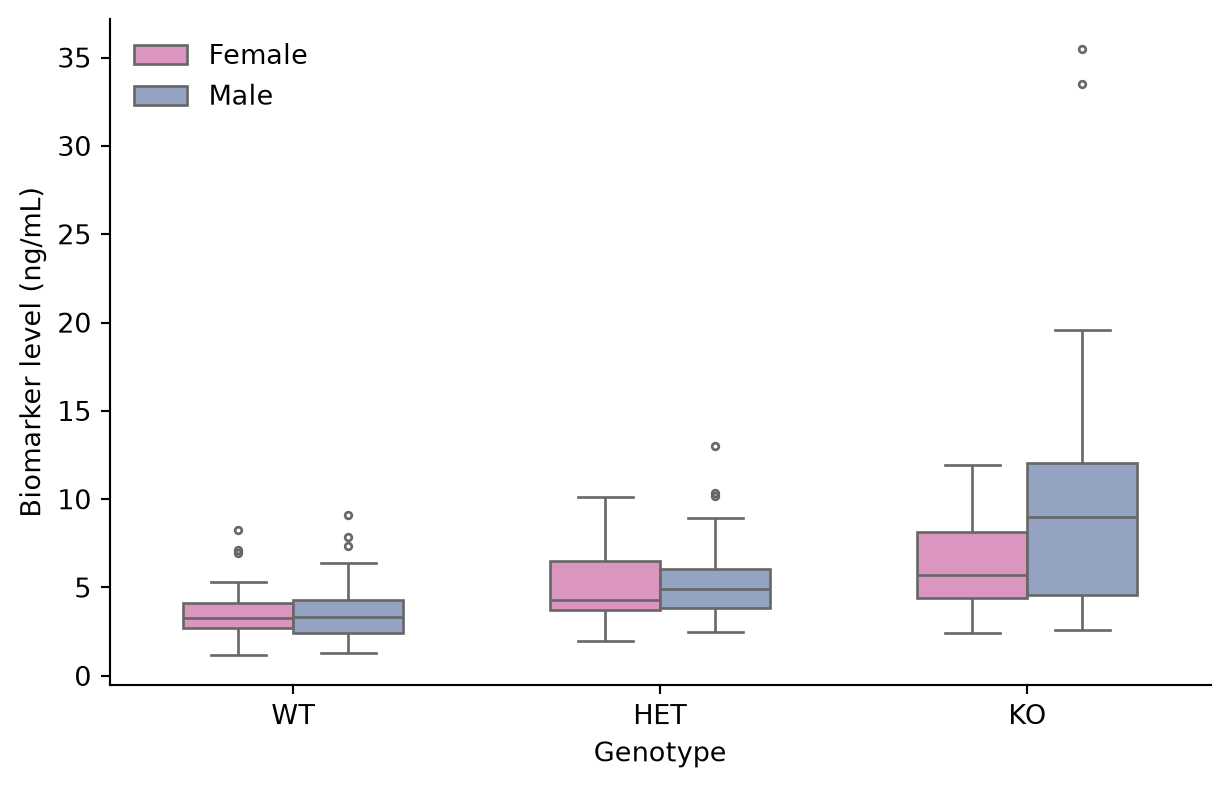

图 3: 引入性别因素的分组箱线图

缺口箱线图

缺口近似中位数的 95% 置信区间；两个箱体之间的缺口不重叠可作为中位数存在差异的非正式证据。

plt.figure(figsize=(5.5, 4.2))
ax = sns.boxplot(data=df, x='Genotype', y='Biomarker',
                 color='#a6d854', width=0.5, linewidth=1.0,
                 notch=True, fliersize=3)
ax.set_xlabel('Genotype')
ax.set_ylabel('Biomarker level (ng/mL)')
ax.spines[['top', 'right']].set_visible(False)
plt.tight_layout()
plt.show()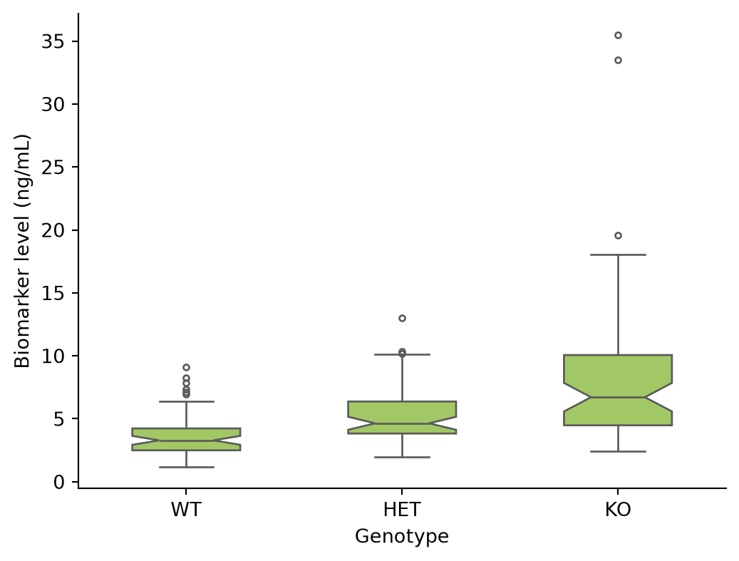

图 4: 缺口箱线图；缺口近似中位数的 95% 置信区间

参考文献

1. Hunter, J. D. (2007). Matplotlib: A 2D graphics environment. Computing in Science & Engineering, 9(3), 90-95.
2. Waskom, M. L. (2021). seaborn: statistical data visualization. Journal of Open Source Software, 6(60), 3021.
3. Spitzer, M., Wildenhain, J., Rappsilber, J., & Tyers, M. (2014). BoxPlotR: a web tool for generation of box plots. Nature Methods, 11(2), 121-122.