美国地图 (县)

作者

[编辑] 郑虎;

[审核] .

注记

Hiplot 网站

本页面为 Hiplot USA Map (County) 插件的源码版本教程，您也可以使用 Hiplot 网站实现无代码绘图，更多信息请查看以下链接:

https://hiplot.cn/basic/map-usa-county?lang=zh_cn

环境配置

系统: Cross-platform (Linux/MacOS/Windows)
编程语言: R
依赖包: ggplot2; RColorBrewer

# 安装包
if (!requireNamespace("ggplot2", quietly = TRUE)) {
  install.packages("ggplot2")
}
if (!requireNamespace("RColorBrewer", quietly = TRUE)) {
  install.packages("RColorBrewer")
}

# 加载包
library(ggplot2)
library(RColorBrewer)

数据准备

# 加载数据
data <- read.delim("files/Hiplot/114-map-usa-county-data.txt", header = T)
dt_map <- readRDS("files/Hiplot/usa.county.rds")

# 整理数据格式
dt_map$Value <- data$value[match(dt_map$county, data$name)]

# 查看数据
head(data)

               name value
1 Lake of the Woods   167
2             Ferry   801
3           Stevens   785
4          Okanogan   783
5      Pend Oreille   796
6          Boundary   126

可视化

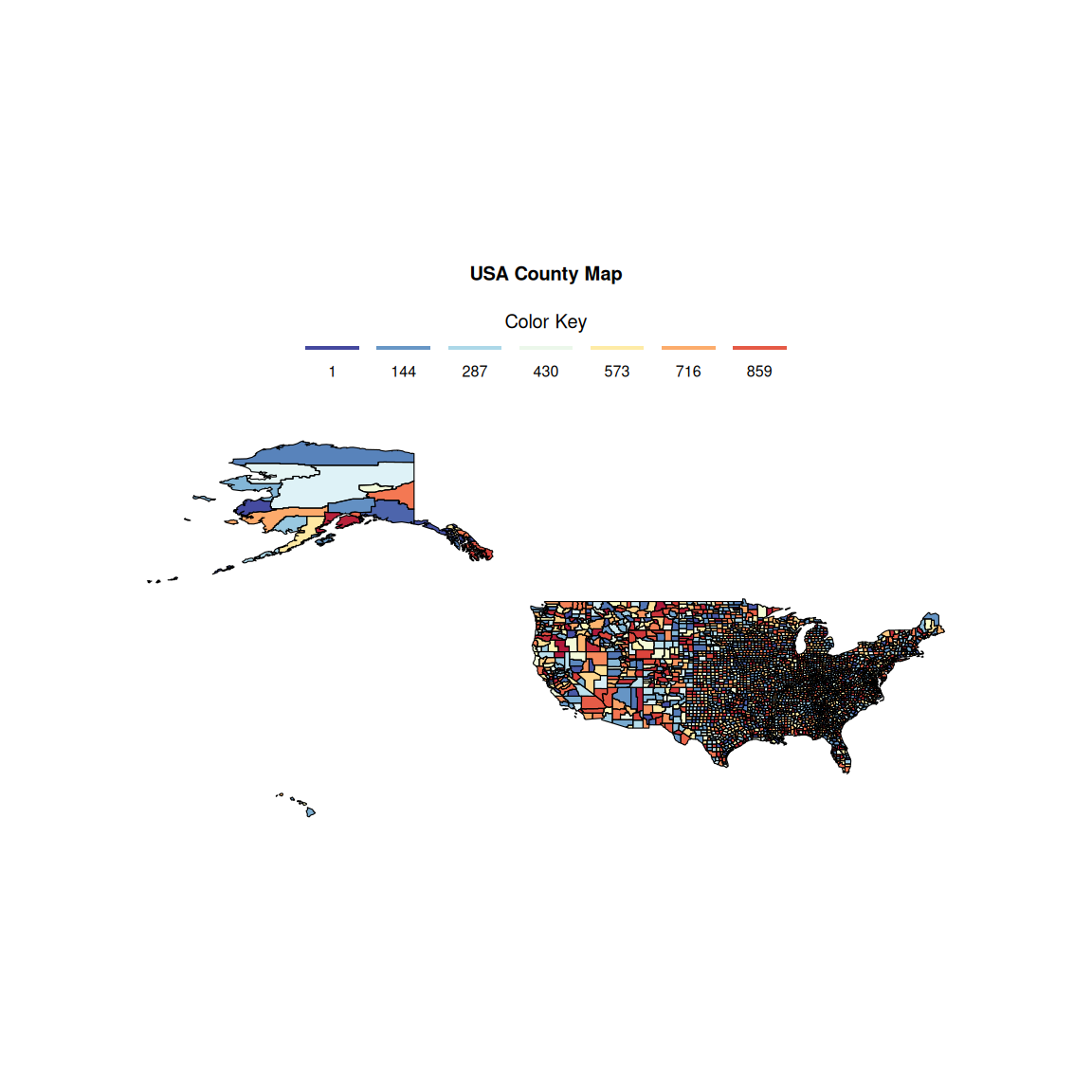
# 美国地图 (县)
p <- ggplot(dt_map) +
  geom_polygon(aes(x = long, y = lat, group = group, fill = Value),
               alpha = 0.9, size = 0.5) +
  geom_path(aes(x = long, y = lat, group = group), color = "black", size = 0.2) +
  scale_fill_gradientn(
    colours = colorRampPalette(rev(brewer.pal(11,"RdYlBu")))(500),
    breaks = seq(min(data$value), max(data$value), 
                 round((max(data$value)-min(data$value))/7)),
    name = "Color Key",
    guide = guide_legend(
      direction = "vertical", keyheight = unit(1, units = "mm"),
      keywidth = unit(8, units = "mm"),
      title.position = "top", title.hjust = 0.5, label.hjust = 0.5,
      nrow = 1, byrow = T, reverse = F, label.position = "bottom")) +
  theme(text = element_text(color = "#3A3F4A"),
        axis.text = element_blank(),
        axis.ticks = element_blank(),
        panel.grid.major = element_blank(),
        panel.grid.minor = element_blank(),
        legend.position = "top",
        legend.text = element_text(size = 4 * 1.5, color = "black"),
        legend.title = element_text(size = 5 * 1.5, color = "black"),
        plot.title = element_text(
          face = "bold", size = 5 * 1.5, hjust = 0.5, 
          margin = margin(t = 4, b = 5), color = "black"),
        plot.background = element_rect(fill = "#FFFFFF", color = "#FFFFFF"),
        panel.background = element_rect(fill = "#FFFFFF", color = NA),
        legend.background = element_rect(fill = "#FFFFFF", color = NA),
        plot.margin = unit(c(1.5, 1.5, 1.5, 1.5), "cm")) +
  labs(x = NULL, y = NULL, title = "USA County Map")

p