ROC 与 PR 曲线（Julia）

🤖 AI Skill — Download the Bizard unified skill for your AI assistant ⬇️ Download Skill ZIP

🔌 MCP Server — Let AI agents (Claude Code, Cursor, …) query Bizard live: claude mcp add bizard -- npx @openbiox/bizard-mcp — or the free hosted instance (no install, faster from mainland China): claude mcp add --transport http bizard http://biotree.top:38123/bizard-mcp/mcp 📖 MCP Docs

📖 Cite Bizard — if Bizard helps your research, please cite: Li, K., Zheng, H., Huang, K., et al. (2026). Bizard: A Community-Driven Platform for Accelerating and Enhancing Biomedical Data Visualization. iMetaMed, e70038. 🔗 DOI / BibTeX

ROC 曲线在所有评分阈值上权衡灵敏度与（1 − 特异度），以 AUC 概括；PR 曲线从阳性类视角审视同一排序，在类别不平衡下是更诚实的展示。曲线本身就是一个阈值扫描——十五行基础 Julia 加 CairoMakie 即可完成。

示例

环境配置

• 系统要求：跨平台（Linux/MacOS/Windows）
• 编程语言：Julia
• 依赖包：CairoMakie、DataFrames、Statistics

using CairoMakie
using DataFrames
using Statistics
using Random

数据准备

我们模拟 2,000 名患者（10% 患病率）的诊断评分：健康人评分以 0 为中心、患者评分整体上移。

Random.seed!(161)

n = 2000; prevalence = 0.10
label = rand(n) .< prevalence
scores = ifelse.(label, 0.9 .+ 0.55 .* randn(n), 0.65 .* randn(n))

function roc_pr_curve(label, scores)
    order = sortperm(scores; rev = true)
    y = label[order]
    tp = cumsum(y); fp = cumsum(.!y)
    P = sum(y); N = length(y) - P
    tpr = tp ./ P
    fpr = fp ./ N
    recall = tpr
    precision = tp ./ (tp .+ fp)
    auc = sum(diff(fpr) .* (tpr[1:end-1] .+ tpr[2:end]) ./ 2)
    ap = sum(precision[i] * (recall[i-1] - recall[i]) for i in 2:length(recall))
    (tpr, fpr, auc, precision, recall, ap)
end
tpr, fpr, auc_value, precision, recall, ap = roc_pr_curve(label, scores)

([0.004524886877828055, 0.00904977375565611, 0.013574660633484163, 0.013574660633484163, 0.01809954751131222, 0.02262443438914027, 0.027149321266968326, 0.03167420814479638, 0.03619909502262444, 0.04072398190045249  …  1.0, 1.0, 1.0, 1.0, 1.0, 1.0, 1.0, 1.0, 1.0, 1.0], [0.0, 0.0, 0.0, 0.0005621135469364812, 0.0005621135469364812, 0.0005621135469364812, 0.0005621135469364812, 0.0005621135469364812, 0.0005621135469364812, 0.0005621135469364812  …  0.9949409780775716, 0.9955030916245081, 0.9960652051714446, 0.9966273187183811, 0.9971894322653176, 0.9977515458122541, 0.9983136593591906, 0.9988757729061271, 0.9994378864530635, 1.0], 0.8686841710351283, [1.0, 1.0, 1.0, 0.75, 0.8, 0.8333333333333334, 0.8571428571428571, 0.875, 0.8888888888888888, 0.9  …  0.11099949773982923, 0.11094377510040161, 0.11088810837932765, 0.11083249749247744, 0.11077694235588972, 0.11072144288577154, 0.11066599899849774, 0.11061061061061062, 0.11055527763881941, 0.1105], [0.004524886877828055, 0.00904977375565611, 0.013574660633484163, 0.013574660633484163, 0.01809954751131222, 0.02262443438914027, 0.027149321266968326, 0.03167420814479638, 0.03619909502262444, 0.04072398190045249  …  1.0, 1.0, 1.0, 1.0, 1.0, 1.0, 1.0, 1.0, 1.0, 1.0], -0.5071316388350325)

可视化

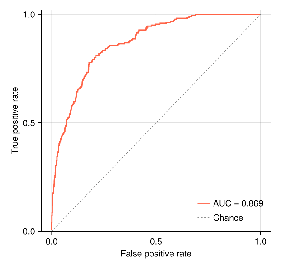
带 AUC 的 ROC 曲线

AUC 用梯形法则沿扫描出的 (FPR, TPR) 路径计算；对角线是随机分类器。

fig = Figure(size = (450, 430))
ax = Axis(fig[1, 1], xlabel = "False positive rate",
          ylabel = "True positive rate")
lines!(ax, fpr, tpr; color = :tomato, linewidth = 1.9,
       label = "AUC = $(round(auc_value; digits = 3))")
lines!(ax, [0, 1], [0, 1]; color = :gray50, linewidth = 0.9,
       linestyle = :dash, label = "Chance")
axislegend(ax; framevisible = false, position = :rb)
ylims!(ax, 0, 1.02)
hidespines!(ax, :t, :r)
fig

图 1: 含机会对角线与梯形 AUC 的 ROC 曲线

精确率–召回率曲线

10% 患病率下，机会精确率位于 0.10（虚线）——ROC 上亮眼的结果在这里可能黯然失色，这正是它的价值。

fig = Figure(size = (450, 430))
ax = Axis(fig[1, 1], xlabel = "Recall", ylabel = "Precision")
lines!(ax, recall, precision; color = :steelblue, linewidth = 1.9,
       label = "AP = $(round(ap; digits = 3))")
hlines!(ax, [prevalence]; color = :gray50, linewidth = 0.9,
        linestyle = :dash, label = "Prevalence = 0.10")
axislegend(ax; framevisible = false, position = :rt)
ylims!(ax, 0, 1.02)
hidespines!(ax, :t, :r)
fig

图 2: 含平均精确率与患病率基线的 PR 曲线

参考文献

1. Fawcett, T. (2006). An introduction to ROC analysis. Pattern Recognition Letters, 27(8), 861-874.
2. Saito, T., & Rehmsmeier, M. (2015). The Precision-Recall Plot Is More Informative than the ROC Plot When Evaluating Binary Classifiers on Imbalanced Datasets. PLoS ONE, 10(3), e0118432.