ROC 与 PR 曲线（Python）

🤖 AI Skill — Download the Bizard unified skill for your AI assistant ⬇️ Download Skill ZIP

🔌 MCP Server — Let AI agents (Claude Code, Cursor, …) query Bizard live: claude mcp add bizard -- npx @openbiox/bizard-mcp — or the free hosted instance (no install, faster from mainland China): claude mcp add --transport http bizard http://biotree.top:38123/bizard-mcp/mcp 📖 MCP Docs

📖 Cite Bizard — if Bizard helps your research, please cite: Li, K., Zheng, H., Huang, K., et al. (2026). Bizard: A Community-Driven Platform for Accelerating and Enhancing Biomedical Data Visualization. iMetaMed, e70038. 🔗 DOI / BibTeX

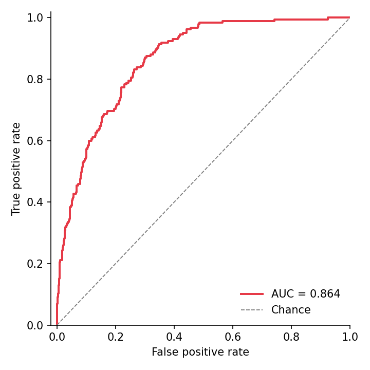
ROC 曲线在所有评分阈值上权衡灵敏度与（1 − 特异度），以 AUC 概括；精确率–召回率（PR）曲线从阳性类视角审视同一排序，在严重类别不平衡下是更诚实的展示。两者都可以从 scikit-learn 的度量函数一次调用获得，再配一行 matplotlib 样式。

示例

环境配置

• 系统要求：跨平台（Linux/MacOS/Windows）
• 编程语言：Python
• 依赖包：matplotlib、seaborn、pandas、numpy、scikit-learn

import matplotlib.pyplot as plt
import seaborn as sns
import pandas as pd
import numpy as np
from sklearn.metrics import roc_curve, auc, precision_recall_curve, average_precision_score

数据准备

我们模拟 2,000 名患者（10% 患病率）的诊断评分：健康人评分以 0 为中心、患者评分整体上移——一个有用但非完美的分类器。

np.random.seed(161)

n, prevalence = 2000, 0.10
label = (np.random.random(n) < prevalence).astype(int)
scores = np.where(label == 1,
                  np.random.normal(0.9, 0.55, n),
                  np.random.normal(0.0, 0.65, n))

fpr, tpr, _ = roc_curve(label, scores)
roc_auc = auc(fpr, tpr)
prec, rec, _ = precision_recall_curve(label, scores)
ap = average_precision_score(label, scores)

可视化

带 AUC 的 ROC 曲线

对角线是随机分类器；把候选模型画在同一坐标上即可一眼完成模型选择。

fig, ax = plt.subplots(figsize=(4.8, 4.8))
ax.plot(fpr, tpr, color='#e63946', linewidth=1.9,
        label=f'AUC = {roc_auc:.3f}')
ax.plot([0, 1], [0, 1], color='0.5', linewidth=0.9, linestyle='--',
        label='Chance')
ax.set_xlabel('False positive rate')
ax.set_ylabel('True positive rate')
ax.set_xlim(-0.02, 1.0)
ax.set_ylim(0, 1.02)
ax.legend(frameon=False, loc='lower right')
ax.spines[['top', 'right']].set_visible(False)
plt.tight_layout()
plt.show()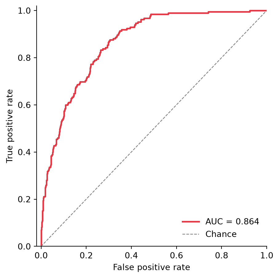

图 1: 含机会对角线与 AUC 的 ROC 曲线

带平均精确率的 PR 曲线

在 10% 患病率下，机会线位于 0.10（虚线）——ROC 上好看到的 AUC 在这里可能黯然失色，这正是 PR 曲线的价值。

fig, ax = plt.subplots(figsize=(4.8, 4.8))
ax.plot(rec, prec, color='#457b9d', linewidth=1.9,
        label=f'AP = {ap:.3f}')
ax.axhline(prevalence, color='0.5', linewidth=0.9, linestyle='--',
           label=f'Prevalence = {prevalence:.2f}')
ax.set_xlabel('Recall')
ax.set_ylabel('Precision')
ax.set_xlim(0, 1.0)
ax.set_ylim(0, 1.02)
ax.legend(frameon=False, loc='upper right')
ax.spines[['top', 'right']].set_visible(False)
plt.tight_layout()
plt.show()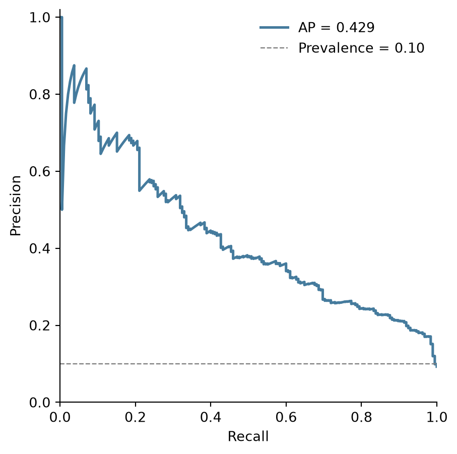

图 2: 含平均精确率与患病率基线的 PR 曲线

参考文献

1. Pedregosa, F., et al. (2011). Scikit-learn: Machine Learning in Python. Journal of Machine Learning Research, 12, 2825-2830.
2. Saito, T., & Rehmsmeier, M. (2015). The Precision-Recall Plot Is More Informative than the ROC Plot When Evaluating Binary Classifiers on Imbalanced Datasets. PLoS ONE, 10(3), e0118432.