import matplotlib.pyplot as plt
import numpy as np
import pandas as pd
from sklearn.calibration import calibration_curve
from sklearn.linear_model import LogisticRegression
from sklearn.model_selection import train_test_split
from dcurves.dca import dca校准曲线与决策曲线 (Python)
临床模型评估套件的 Python 对应版本(ROC 见 ROC & PR (Python);校准与 DCA 的 R 版见校准曲线与决策曲线)。区分度(AUC)说明模型排序正确;校准说明其概率值得信任——预测为 30% 的患者中是否真的有约 30% 发生事件?决策曲线分析(DCA)再问临床问题:在哪个风险阈值上按模型行动比”全部治疗”或”全部不治”让更多患者获益 [1]。TRIPOD 式报告要求三者齐备。
本教程涵盖两种工作流:
- 两个 logistic 模型的校准曲线(
sklearn.calibration.calibration_curve()); -
dcurves包的净受益决策曲线——MSKCC 实现的 Vickers DCA [2]——以及 treat-all/treat-none 参照。
Example
Setup
- 系统要求:跨平台(Linux/MacOS/Windows)
- 编程语言:Python
- 依赖包:
matplotlib、numpy、pandas、scikit-learn、dcurves
Data Preparation
模拟 800 例患者、二分类 1 年终点、三个预测因子的队列;在训练集上拟合完整与简化两个 logistic 模型,在留出的 40% 上评估——校准必须在与建模无关的数据上判断。
rng = np.random.default_rng(418)

m = 800
age = rng.normal(60, 12, m)
ecog = rng.integers(0, 3, m)
marker = rng.normal(0, 1, m)
lp = -1.2 + 0.03 * (age - 60) + 0.5 * ecog + 0.8 * marker
y1y = rng.binomial(1, 1 / (1 + np.exp(-lp)))

df = pd.DataFrame({"age": age, "ecog": ecog, "marker": marker, "y": y1y})
tr, te = train_test_split(df, test_size=0.4, random_state=251, stratify=df.y)

m_full = LogisticRegression().fit(tr[["age", "ecog", "marker"]], tr.y)
m_simple = LogisticRegression().fit(tr[["ecog"]], tr.y)
te = te.assign(p_full=m_full.predict_proba(te[["age", "ecog", "marker"]])[:, 1],
               p_simple=m_simple.predict_proba(te[["ecog"]])[:, 1])
te.y.mean().round(3)np.float64(0.353)Visualization
1. 校准曲线
fig, ax = plt.subplots(figsize=(5.6, 4.6))
for name, col, c in [("Full model", "p_full", "#2166AC"),
                     ("Simple model", "p_simple", "#B2182B")]:
    prob_true, prob_pred = calibration_curve(te.y, te[col], n_bins=8,
                                             strategy="quantile")
    ax.plot(prob_pred, prob_true, "o-", color=c, label=name, markersize=4)
ax.plot([0, 1], [0, 1], "k--", lw=0.8)
ax.set_xlabel("Predicted probability")
ax.set_ylabel("Observed proportion")
ax.set_title("Calibration curves (quantile bins)")
ax.legend(loc="upper left")
fig.tight_layout()
plt.show()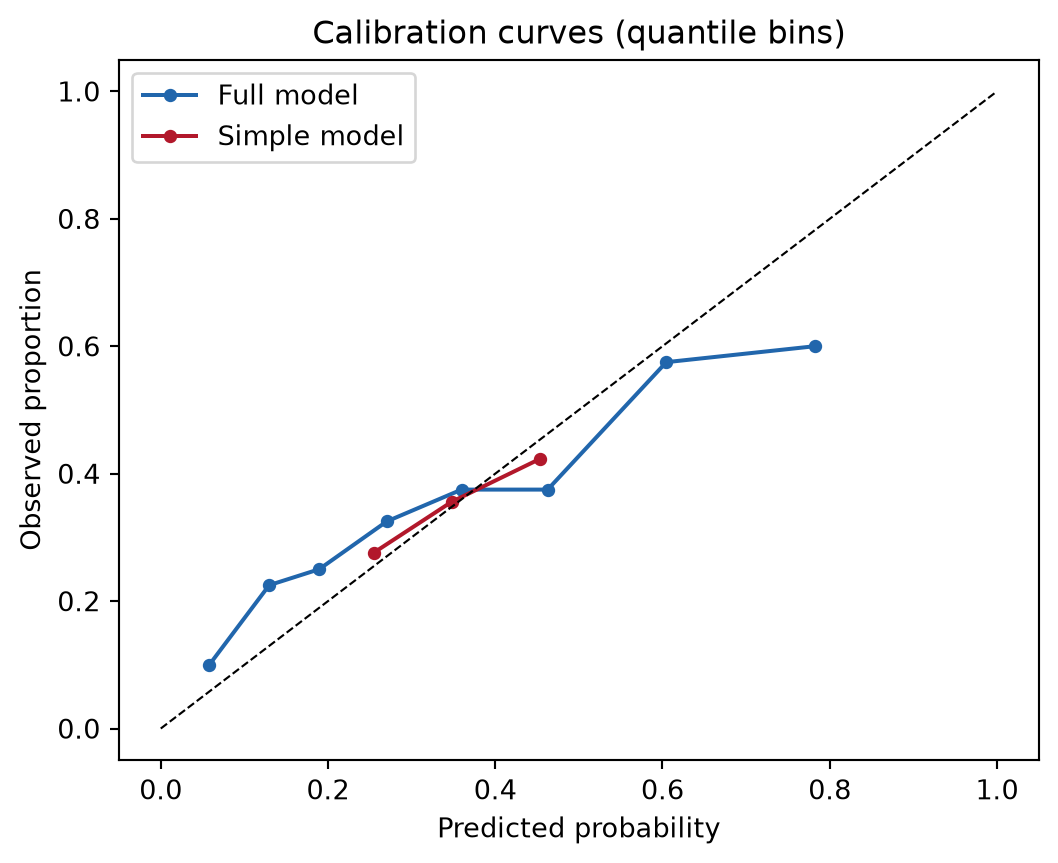
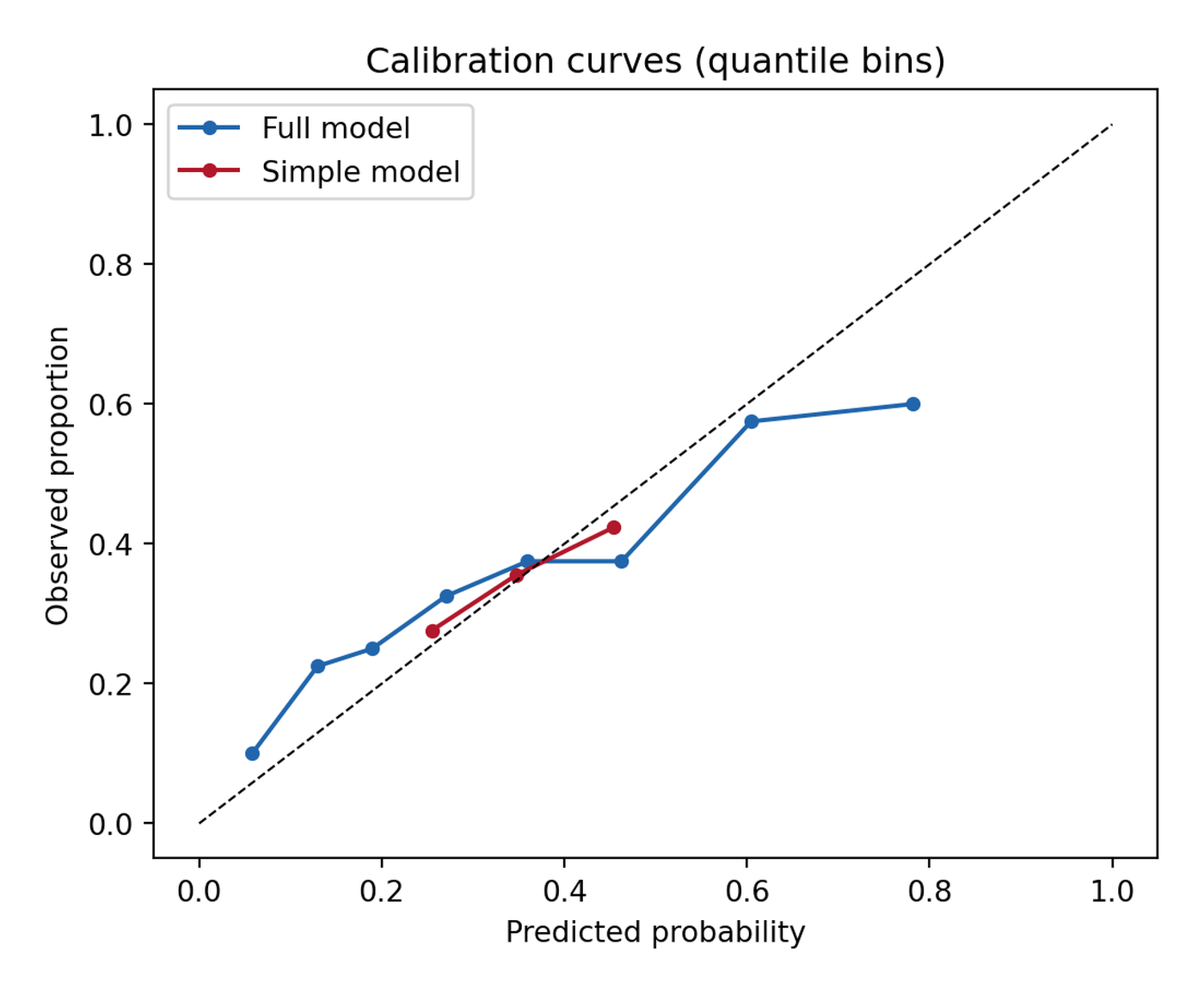
对角线下方意味着模型高估。strategy="quantile" 保证每个分箱都有样本(等宽分箱的尾部会空箱);报告分箱数,Brier 分数可把同一信息压缩成一个数。
2. 决策曲线分析
d = dca(data=te, outcome="y", modelnames=["p_full", "p_simple"],
        thresholds=np.arange(0.01, 0.99, 0.01))
net = d  # 整洁数据框:model / threshold / net_benefit / net_intervention_avoided

fig, ax = plt.subplots(figsize=(5.8, 4.6))
for label, c in [("p_full", "#2166AC"), ("p_simple", "#B2182B")]:
    sub = net[net.model == label]
    ax.plot(sub.threshold, sub.net_benefit, color=c, label=label)
ax.axhline(0, color="grey", lw=0.8)
allpos = net[net.model == "all"]
ax.plot(allpos.threshold, allpos.net_benefit, color="grey", ls=":", label="Treat all")
ax.set_xlabel("Threshold probability")
ax.set_ylabel("Net benefit")
ax.set_title("Decision curve analysis (dcurves)")
ax.set_ylim(-0.05, 0.45)
ax.legend()
fig.tight_layout()
plt.show()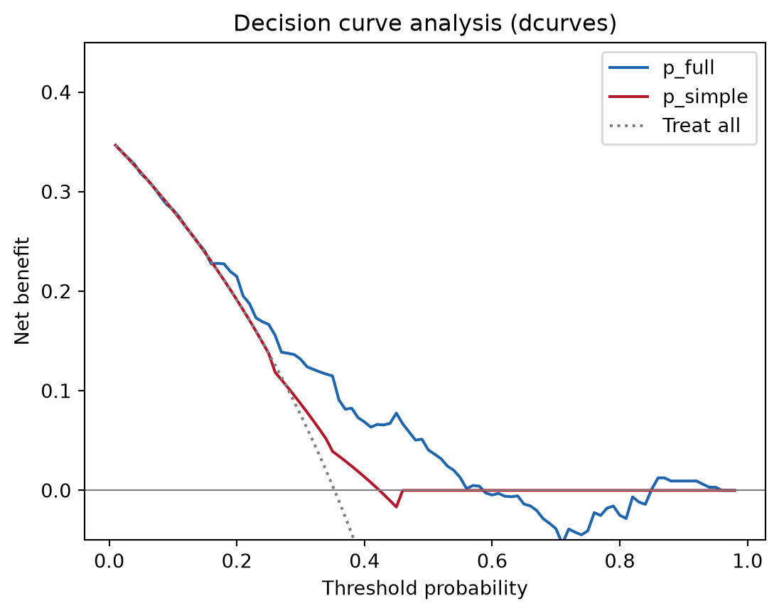
净受益 = (真阳性 − 假阳性 × 阈值赔率) / n:在每个临床阈值上用一个假阳性的代价折算真阳性。模型的有用区间是其曲线同时高于 treat-all 与 treat-none 的范围——本例约在 10%–55%。
提示实践要点
-
dca()返回整洁数据框(列含model、threshold、net_benefit、net_intervention_avoided)——需要期刊样式时直接用它画图,而非包内置的 matplotlib 后端。 - “Treat all”(
model == "all")与 treat-none(净受益 0)是两条必画参照;模型若从不优于二者,无论 AUC 多高都没有决策价值。 - 训练集上的校准是乐观的——始终在留出集或交叉验证预测(
sklearn.model_selection.cross_val_predict)上评估。 - 生存终点时
dcurves.dca接受time/time_in_censor参数;在同一图中混合二分类与时间-事件曲线前先读包 vignette。
Application
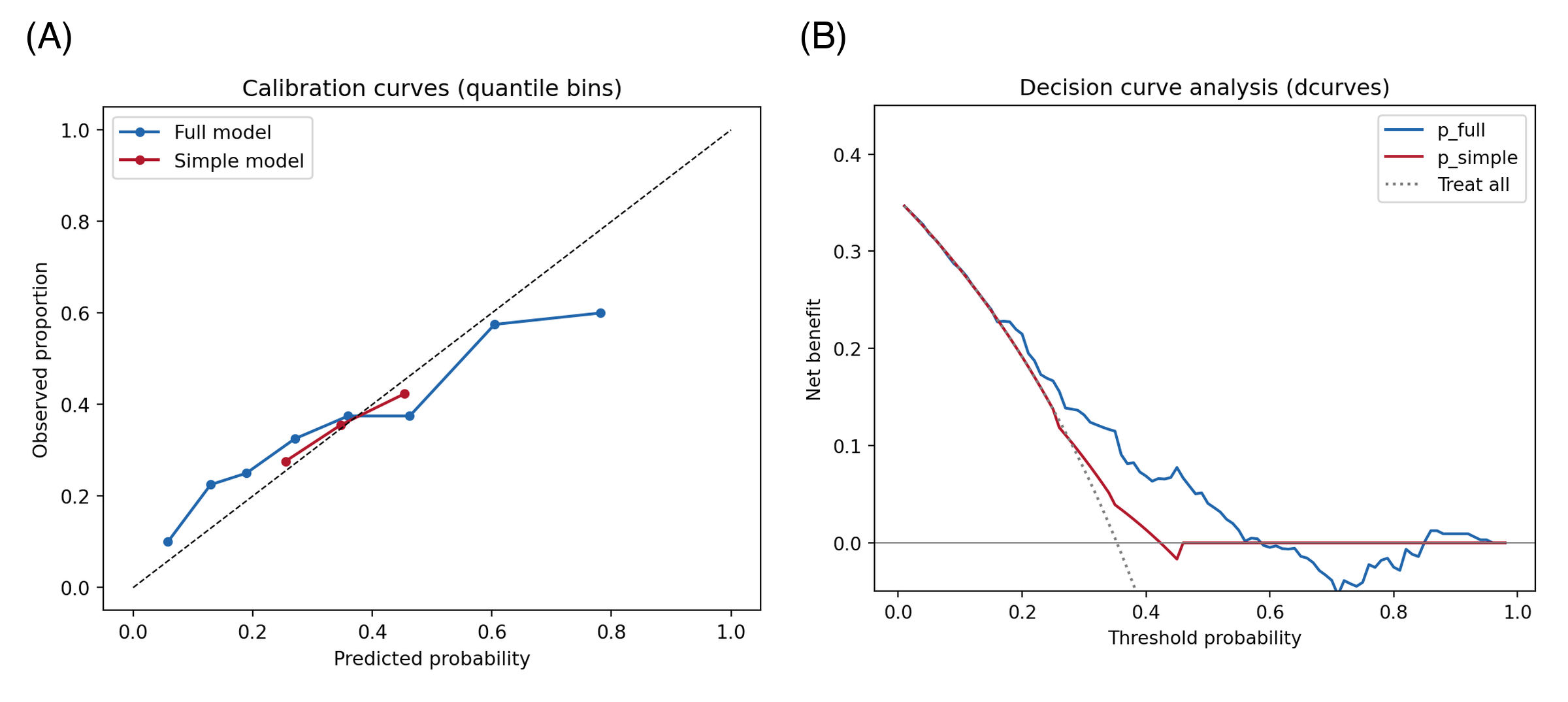
校准 + DCA 组合出现在临床预测模型论文(与 ROC 并列)、医学 AI 摘要(TRIPOD-AI 要求两者)以及把运行阈值视为政策选择的模型选型备忘中。下图模拟典型论文版式:(A) 校准曲线与 (B) 净受益决策曲线。
Reference
[1] Vickers AJ, Elkin EB. Decision curve analysis: a novel method for evaluating prediction models. Med Decis Making. 2006;26(6):565-574. doi:10.1177/0272989X06295361
[2] Vickers AJ, van Calster B, Steyerberg EW. A simple, step-by-step guide to interpreting decision curve analysis. Diagn Progn Res. 2019;3:18. doi:10.1186/s41512-019-0064-7
[3] Van Calster B, McLernon DJ, van Smeden M, et al. Calibration: the Achilles heel of predictive analytics. BMC Med. 2019;17:230. doi:10.1186/s12916-019-1466-7