using CairoMakie
using DataFrames
using Statistics
using Random相关矩阵图(Julia)
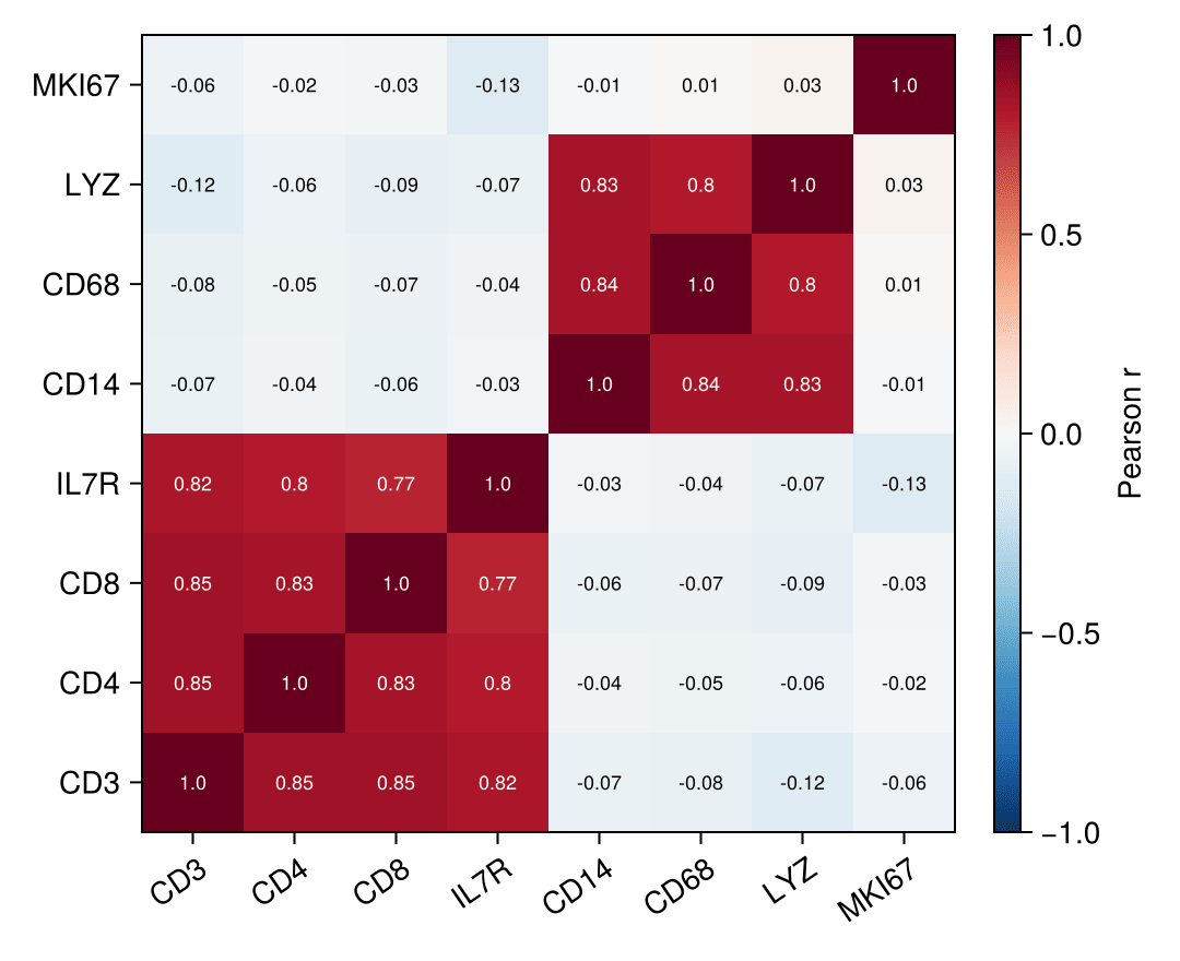
相关矩阵图把特征面板的两两相关系数编码为彩色矩阵单元格,一眼读出共表达模块与冗余标志物。在生物医学研究中,它是标志物面板的常规 QC。Julia 的 Statistics.cor 计算矩阵,CairoMakie.heatmap! 渲染,并通过 text! 逐格标注数值。
示例
环境配置
- 系统要求:跨平台(Linux/MacOS/Windows)
- 编程语言:Julia
- 依赖包:
CairoMakie、DataFrames、Statistics
数据准备
我们模拟一个含两个相关模块(T 细胞标志物与髓系标志物)加一个弱相关增殖评分的 8 标志物免疫面板,并计算 Pearson 矩阵。
Random.seed!(101)

n = 250
latent_t = randn(n)
latent_m = randn(n)
panel = DataFrame(
    CD3   = latent_t .+ 0.4 .* randn(n),
    CD4   = latent_t .+ 0.5 .* randn(n),
    CD8   = latent_t .+ 0.5 .* randn(n),
    IL7R  = latent_t .+ 0.6 .* randn(n),
    CD14  = latent_m .+ 0.4 .* randn(n),
    CD68  = latent_m .+ 0.5 .* randn(n),
    LYZ   = latent_m .+ 0.5 .* randn(n),
    MKI67 = randn(n))
markers = names(panel)
corr = Matrix(cor(Matrix(panel)))
8×8 Matrix{Float64}:
1.0 0.847918 0.851106 … -0.0763281 -0.121005 -0.0607499
0.847918 1.0 0.830831 -0.0535264 -0.0561228 -0.0197228
0.851106 0.830831 1.0 -0.0657583 -0.0852999 -0.0260574
0.817423 0.795928 0.77068 -0.0428039 -0.0724778 -0.129194
-0.0678254 -0.0418892 -0.0612808 0.835868 0.832141 -0.00942036
-0.0763281 -0.0535264 -0.0657583 … 1.0 0.803521 0.0111169
-0.121005 -0.0561228 -0.0852999 0.803521 1.0 0.0349363
-0.0607499 -0.0197228 -0.0260574 0.0111169 0.0349363 1.0可视化
带标注的相关热图
使用反转的发散色图(红=正相关)、固定 ±1 的 colorrange 保证跨研究可比,并用 text! 逐格标注数值。
fig = Figure(size = (540, 440))
ax = Axis(fig[1, 1]; xticks = (1:8, markers), yticks = (1:8, markers),
          xticklabelrotation = 0.6)
hm = heatmap!(ax, corr; colormap = Reverse(:RdBu), colorrange = (-1, 1))
for i in 1:8, j in 1:8
    text!(ax, j, i; text = string(round(corr[i, j]; digits = 2)),
          align = (:center, :center), fontsize = 9,
          color = abs(corr[i, j]) > 0.55 ? :white : :black)
end
Colorbar(fig[1, 2], hm; label = "Pearson r")
fig
下三角相关矩阵图
用 NaN 掩掉镜像上三角去除冗余;nan_color 让空格保持不可见。
corr_masked = [i < j ? NaN : corr[i, j] for i in 1:8, j in 1:8]

fig = Figure(size = (460, 420))
ax = Axis(fig[1, 1]; xticks = (1:8, markers), yticks = (1:8, markers),
          xticklabelrotation = 0.6)
heatmap!(ax, corr_masked; colormap = Reverse(:RdBu), colorrange = (-1, 1),
         nan_color = :white)
for i in 1:8, j in 1:i
    text!(ax, j, i; text = string(round(corr[i, j]; digits = 2)),
          align = (:center, :center), fontsize = 9,
          color = abs(corr[i, j]) > 0.55 ? :white : :black)
end
hidespines!(ax)
fig
参考文献
- Makie development team. Makie.jl documentation — heatmap. https://docs.makie.org/stable/reference/plots/heatmap
- Danisch, S., & Krumbiegel, J. (2021). Makie.jl: Flexible high-performance data visualization for Julia. Journal of Open Source Software, 6(65), 3349.