using CairoMakie
using DataFrames
using Statistics
using Random棒棒糖图与哑铃图(Julia)
棒棒糖图用细线加端点圆点替代条形图的条形,在保持排序可读性的同时大幅削减图形墨量;哑铃图把每行两个圆点用线段连接,直观呈现两个条件间的变化。在生物医学研究中,棒棒糖图常用于富集条目或效应量排序,哑铃图用于逐特征比较两个队列或处理臂。二者均由 CairoMakie 的 hlines!/vlines! 与 scatter! 组合而成。
示例
环境配置
- 系统要求:跨平台(Linux/MacOS/Windows)
- 编程语言:Julia
- 依赖包:
CairoMakie、DataFrames、Statistics
数据准备
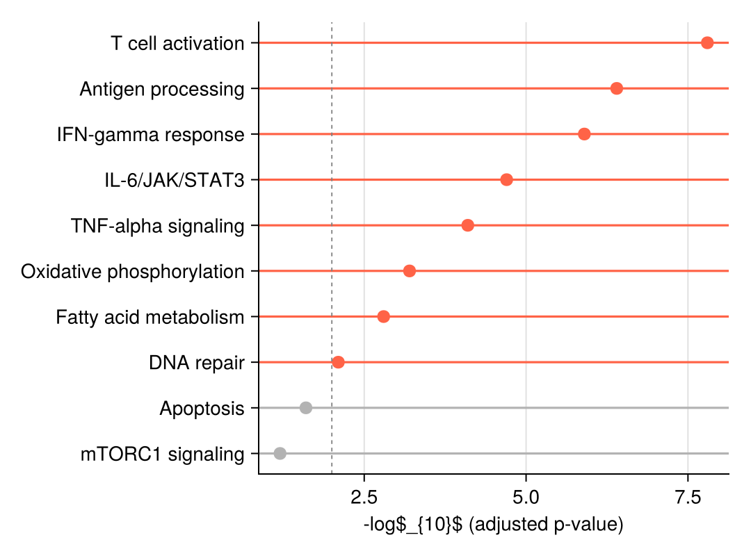
我们模拟一个通路富集结果(基因集的 −log10 校正 p 值)和一张用于哑铃图的两条件差异表达表。
pathways = ["T cell activation", "Antigen processing", "IFN-gamma response",
            "IL-6/JAK/STAT3", "TNF-alpha signaling", "Oxidative phosphorylation",
            "Fatty acid metabolism", "DNA repair", "Apoptosis", "mTORC1 signaling"]
enrichment = DataFrame(Pathway = pathways,
                       NegLogFDR = [7.8, 6.4, 5.9, 4.7, 4.1, 3.2, 2.8, 2.1, 1.6, 1.2])
sort!(enrichment, :NegLogFDR)

dumbbell = DataFrame(Gene = ["CD274", "IFIT1", "CXCL10", "MKI67", "STAT1"],
                     Sham = [-0.3, 2.1, 2.8, 0.5, 1.9],
                     Treat = [1.4, 3.9, 4.6, -1.2, 3.3])
sort!(dumbbell, :Treat)
5×3 DataFrame
| Row | Gene | Sham | Treat |
|---|---|---|---|
| String | Float64 | Float64 | |
| 1 | MKI67 | 0.5 | -1.2 |
| 2 | CD274 | -0.3 | 1.4 |
| 3 | STAT1 | 1.9 | 3.3 |
| 4 | IFIT1 | 2.1 | 3.9 |
| 5 | CXCL10 | 2.8 | 4.6 |
可视化
横向棒棒糖图
每行为一条线段(hlines!)加一个标记(scatter!);显著条目用颜色高亮并配阈值参考线。
y_pos = 1:nrow(enrichment)
sig = enrichment.NegLogFDR .>= 2
dot_colors = ifelse.(sig, :tomato, :gray70)

fig = Figure(size = (540, 400))
ax = Axis(fig[1, 1], xlabel = "-log\$_{10}\$ (adjusted p-value)")
hlines!(ax, y_pos; xmin = 0.0, xmax = enrichment.NegLogFDR,
        color = dot_colors, linewidth = 1.6)
scatter!(ax, enrichment.NegLogFDR, y_pos; color = dot_colors, markersize = 13)
vlines!(ax, [2]; color = :gray50, linestyle = :dash, linewidth = 0.9)
ax.yticks = (y_pos, enrichment.Pathway)
hidespines!(ax, :t, :r)
fig
纵向棒棒糖图
同样的构造用 vlines! 旋转为纵向,适合标签较短或幻灯片场景。
top8 = enrichment[end-7:end, :]

fig = Figure(size = (540, 380))
ax = Axis(fig[1, 1], ylabel = "-log\$_{10}\$ (adjusted p-value)")
x_pos = 1:nrow(top8)
vlines!(ax, x_pos; ymin = 0.0, ymax = top8.NegLogFDR,
        color = :steelblue, linewidth = 1.6)
scatter!(ax, x_pos, top8.NegLogFDR; color = :steelblue, markersize = 13)
ax.xticks = (x_pos, top8.Pathway)
ax.xticklabelrotation = 0.7
hidespines!(ax, :t, :r)
fig
哑铃图
每个特征一条线段连接两个条件的值;两端圆点按条件着色,使变化的方向与幅度一目了然。
y = 1:nrow(dumbbell)

fig = Figure(size = (540, 380))
ax = Axis(fig[1, 1], xlabel = "log\$_{2}\$ fold change")
hlines!(ax, y; xmin = min.(dumbbell.Sham, dumbbell.Treat),
        xmax = max.(dumbbell.Sham, dumbbell.Treat),
        color = :gray70, linewidth = 2)
scatter!(ax, dumbbell.Sham, y; color = :steelblue, markersize = 13, label = "Sham")
scatter!(ax, dumbbell.Treat, y; color = :tomato, markersize = 13, label = "Treatment")
vlines!(ax, [0]; color = :gray40, linewidth = 0.9)
axislegend(ax; framevisible = false, position = :rb)
ax.yticks = (y, dumbbell.Gene)
hidespines!(ax, :t, :r)
fig
参考文献
- Makie development team. Makie.jl documentation — linesegments, scatter. https://docs.makie.org/stable/reference/plots/linesegments
- From Data to Viz. Lollipop plot. https://www.data-to-viz.com/graph/lollipop.html