# 安装包
if (!requireNamespace("readr", quietly = TRUE)) {
  install.packages("readr")
}
if (!requireNamespace("ggplot2", quietly = TRUE)) {
  install.packages("ggplot2")
}
if (!requireNamespace("ggExtra", quietly = TRUE)) {
  install.packages("ggExtra")
}
if (!requireNamespace("tidyverse", quietly = TRUE)) {
  install.packages("tidyverse")
}
if (!requireNamespace("cowplot", quietly = TRUE)) {
  install.packages("cowplot")
}
if (!requireNamespace("viridis", quietly = TRUE)) {
  install.packages("viridis")
}
if (!requireNamespace("ggpmisc", quietly = TRUE)) {
  install.packages("ggpmisc")
}
if (!requireNamespace("ggpubr", quietly = TRUE)) {
  install.packages("ggpubr")
}

# 加载包
library(readr)      # 读取 tsv 文件
library(ggplot2)    # 用于创建图
library(ggExtra)    # 用于增强 ggplot2 图形
library(tidyverse)  # 用于获取数据操作功能
library(cowplot)    # 用于将单独的 ggplot 合并到同一张图形中
library(viridis)    # 用于颜色映射
library(ggpmisc)    # ggplot2 的扩展,包含用于统计注释的附加函数
library(ggpubr) # ggplot2 的扩展,添加了可发布的主题、排列多个图表和统计测试直方图
直方图(histogram)用直条矩形面积代表各组频数,各矩形面积总和代表频数的总和。它主要用于表示连续变量频数分布情况。
示例
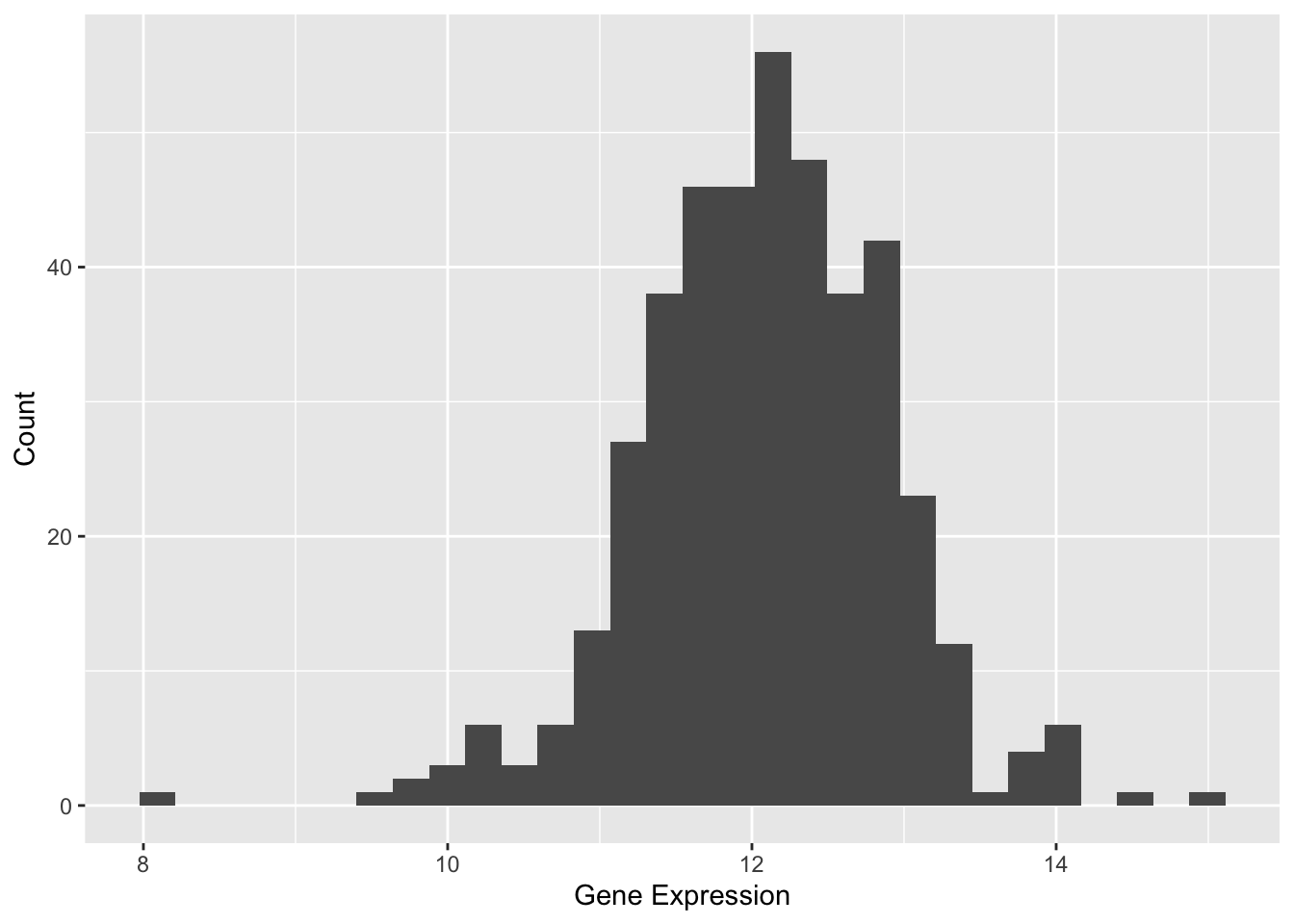
这个基础直方图展示了不同样本中TSPAN6基因的表达水平。x轴表示数据值,每个条形代表一个特定的值范围;y轴表示该范围内的数据点数量。在这个直方图中,条形表示每个指定范围内的值的数量。
直方图显示数据以值12为中心,值的范围大致为8到16。直方图的形状近似于钟形,表明数据可能遵循正态分布。
环境配置
系统要求: 跨平台(Linux/MacOS/Windows)
编程语言:R
依赖包:
readr,ggplot2,ggExtra,tidyverse,cowplot,viridis,ggpmisc,ggpubr
sessioninfo::session_info("attached")─ Session info ───────────────────────────────────────────────────────────────
setting value
version R version 4.6.0 (2026-04-24)
os Ubuntu 24.04.4 LTS
system x86_64, linux-gnu
ui X11
language (EN)
collate C.UTF-8
ctype C.UTF-8
tz UTC
date 2026-05-09
pandoc 3.1.3 @ /usr/bin/ (via rmarkdown)
quarto 1.9.37 @ /usr/local/bin/quarto
─ Packages ───────────────────────────────────────────────────────────────────
package * version date (UTC) lib source
cowplot * 1.2.0 2025-07-07 [1] RSPM
dplyr * 1.2.1 2026-04-03 [1] RSPM
forcats * 1.0.1 2025-09-25 [1] RSPM
ggExtra * 0.11.0 2025-09-01 [1] RSPM
ggplot2 * 4.0.3.9000 2026-05-04 [1] Github (tidyverse/ggplot2@6870419)
ggpmisc * 0.7.0 2026-03-23 [1] RSPM
ggpp * 0.6.0 2026-01-18 [1] RSPM
ggpubr * 0.6.3 2026-02-24 [1] RSPM
lubridate * 1.9.5 2026-02-04 [1] RSPM
purrr * 1.2.2 2026-04-10 [1] RSPM
readr * 2.2.0 2026-02-19 [1] RSPM
stringr * 1.6.0 2025-11-04 [1] RSPM
tibble * 3.3.1 2026-01-11 [1] RSPM
tidyr * 1.3.2 2025-12-19 [1] RSPM
tidyverse * 2.0.0 2023-02-22 [1] RSPM
viridis * 0.6.5 2024-01-29 [1] RSPM
viridisLite * 0.4.3 2026-02-04 [1] RSPM
[1] /home/runner/work/_temp/Library
[2] /opt/R/4.6.0/lib/R/site-library
[3] /opt/R/4.6.0/lib/R/library
* ── Packages attached to the search path.
──────────────────────────────────────────────────────────────────────────────数据准备
我们使用内置的 R 数据集(iris、mtcars)以及来自UCSC Xena DATASETS的TCGA-BRCA.htseq_counts.tsv数据集。所选基因仅用于演示目的。
# 读取 TSV 数据
data <- readr::read_csv("https://bizard-1301043367.cos.ap-guangzhou.myqcloud.com/TCGA-LIHC.htseq_counts.csv.gz")

# 过滤并重塑第一个基因 TSPAN6 的数据(Ensembl ID:ENSG00000000003.13)
data1 <- data %>%
  filter(Ensembl_ID == "ENSG00000000003.13") %>%
  pivot_longer(
    cols = -Ensembl_ID,
    names_to = "sample",
    values_to = "expression"
  ) %>%
  mutate(var = "var1")  # 添加一列来区分变量

# 过滤并重塑第二个基因 SCYL3 的数据(Ensembl ID:ENSG00000000457.12)
data2 <- data %>%
  filter(Ensembl_ID == "ENSG00000000457.12") %>%
  pivot_longer(
    cols = -Ensembl_ID,
    names_to = "sample",
    values_to = "expression"
  ) %>%
  mutate(var = "var2")  # 添加一列来区分变量

# 合并两个数据集
data12 <- bind_rows(data1, data2)

# 查看最终合并的数据集
head(data12)
# A tibble: 6 × 4
Ensembl_ID sample expression var
<chr> <chr> <dbl> <chr>
1 ENSG00000000003.13 TCGA-DD-A4NG-01A 12.8 var1
2 ENSG00000000003.13 TCGA-G3-AAV4-01A 9.72 var1
3 ENSG00000000003.13 TCGA-2Y-A9H1-01A 11.3 var1
4 ENSG00000000003.13 TCGA-CC-A3M9-01A 11.6 var1
5 ENSG00000000003.13 TCGA-K7-AAU7-01A 11.5 var1
6 ENSG00000000003.13 TCGA-BC-A10W-01A 12.0 var1 可视化
1. 基础直方图
图 1 展示了 TSPAN6 基因在不同样本中的表达量分布情况。
# 基础直方图
p1 <- ggplot(data1, aes(x = expression)) +
  geom_histogram() +
  labs(x = "Gene Expression", y = "Count")

p1
提示
关键参数: binwidth / bins
binwidth/bins参数决定每一个箱体包含数据的多少,改变binwidth/bins会对图形造成很大的影响,也会影响到想要表达的信息。
p2_1 <- ggplot(data1, aes(x = expression)) +
  geom_histogram(bins = 30, fill = "skyblue", color = "white") +
  ggtitle("Bins = 30") +
  labs(x = "Gene Expression", y = "Count")

p2_2 <- ggplot(data1, aes(x = expression)) +
  geom_histogram(bins = 50, fill = "skyblue", color = "white") +
  ggtitle("Bins = 50") +
  labs(x = "Gene Expression", y = "Count")

cowplot::plot_grid(p2_1, p2_2)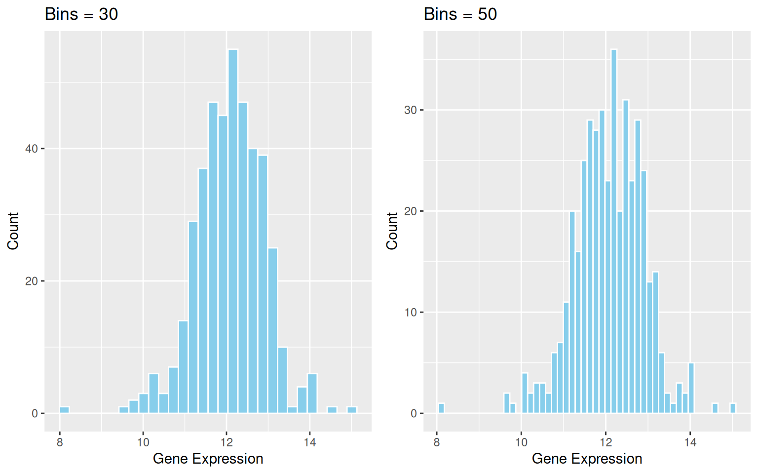
binwidth / bins
2. 添加密度曲线的直方图
密度曲线则提供了数据分布的平滑表示,它不依赖于具体的分箱数,而是使用核密度估计(kernel density estimation)来平滑分布曲线。这样可以更好地展示数据的总体趋势和形状。
p1 <- ggplot(data1, aes(x = expression)) +
  geom_histogram(aes(y = after_stat(density)), bins = 30, fill = "skyblue", color = "white") +
  geom_density(alpha = 0.2, fill = "#FF6666") +
  labs(x = "Gene Expression", y = "Density")

p1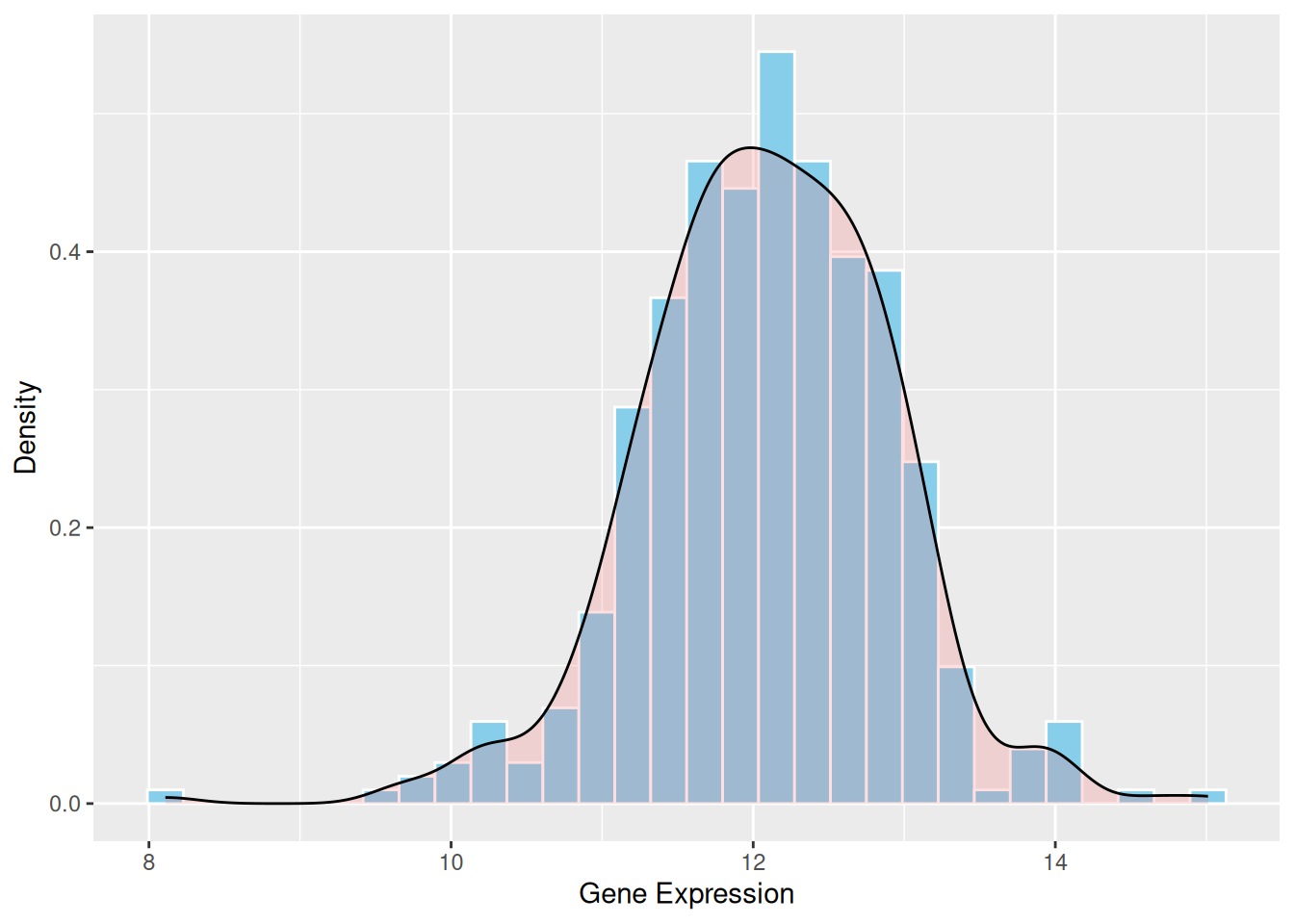
3. 镜像直方图
镜像直方图帮助我们非常直观地对比两个数据集的分布。通过镜像结构,可以快速判断两个数据集是否存在对称性或差异。镜像直方图将两个直方图整合在一张图上,减少了所需的可视化空间,同时保持了对数据分布的清晰描述。
p <- ggplot(data12, aes(x = expression, fill = var)) +
  geom_histogram(data = subset(data12, var == "var1"),
                 aes(y = after_stat(density)),
                 binwidth = 0.5,
                 alpha = 0.7,
                 fill = "#69b3a2") +
  geom_histogram(data = subset(data12, var == "var2"),
                 aes(y = -after_stat(density)),
                 binwidth = 0.5,
                 alpha = 0.7,
                 fill = "#404080") +
  scale_fill_manual(values = c("var1" = "#69b3a2", "var2" = "#404080")) +
  labs(x = "Gene Expression", y = "Density")

p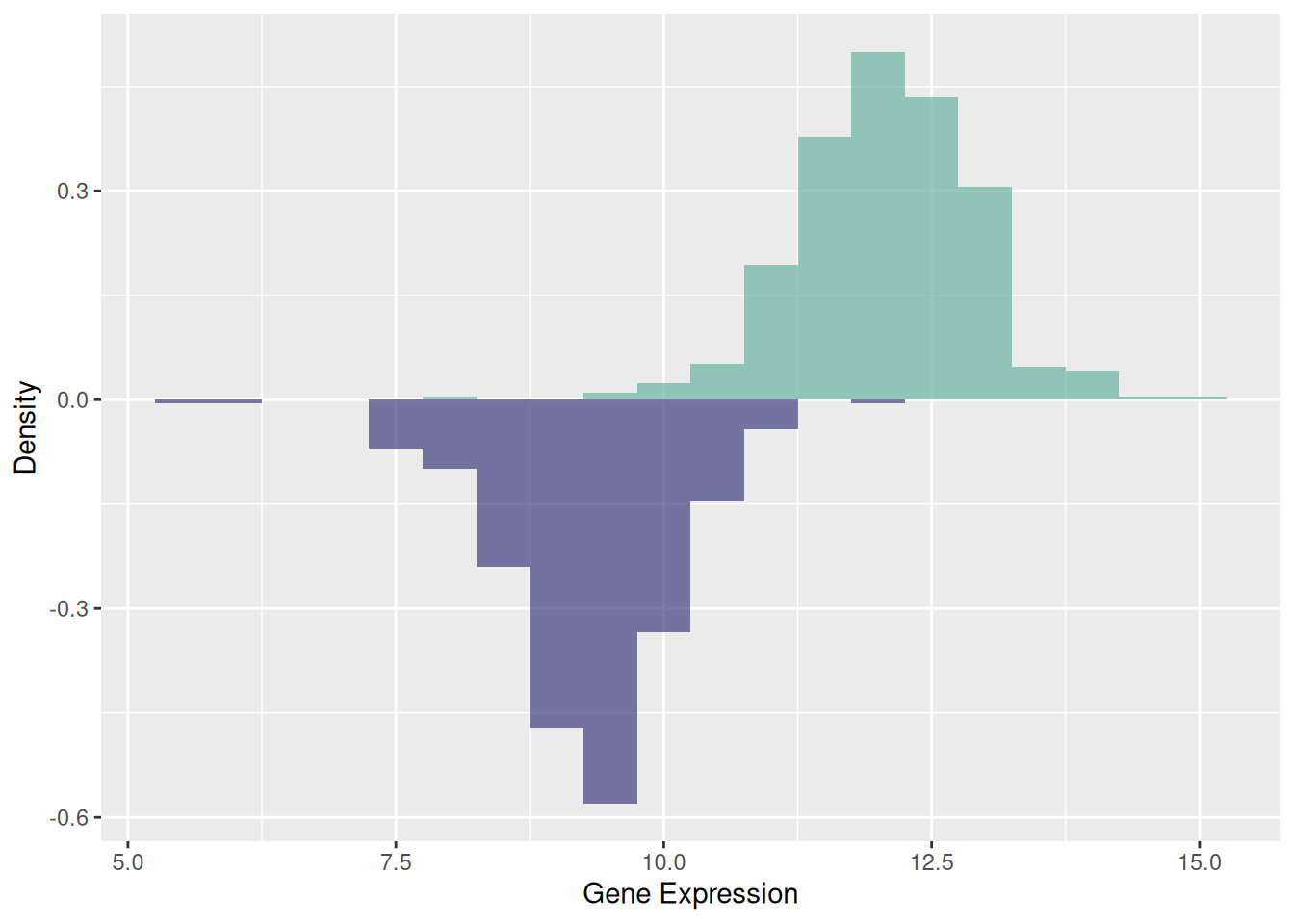
4.同一轴上的多个直方图
同一轴上叠加或并排的直方图允许我们在同一个坐标系内,直接对比两个或多个数据集的分布。通过颜色或透明度的设置,可以在同一图中清楚地看到数据的重叠区域以及不同数据的分布差异。用于2~3组数据,过多会导致图片混乱难以阅读。
p <- data12 %>%
  ggplot(aes(x = expression, fill = var)) +
  geom_histogram(color = "#e9ecef", alpha = 0.6, position = 'identity') +
  scale_fill_manual(values = c("#69b3a2", "#404080")) +
  labs(x = "Expression Value", y = "Count", fill = "Type") +
  theme_minimal()

p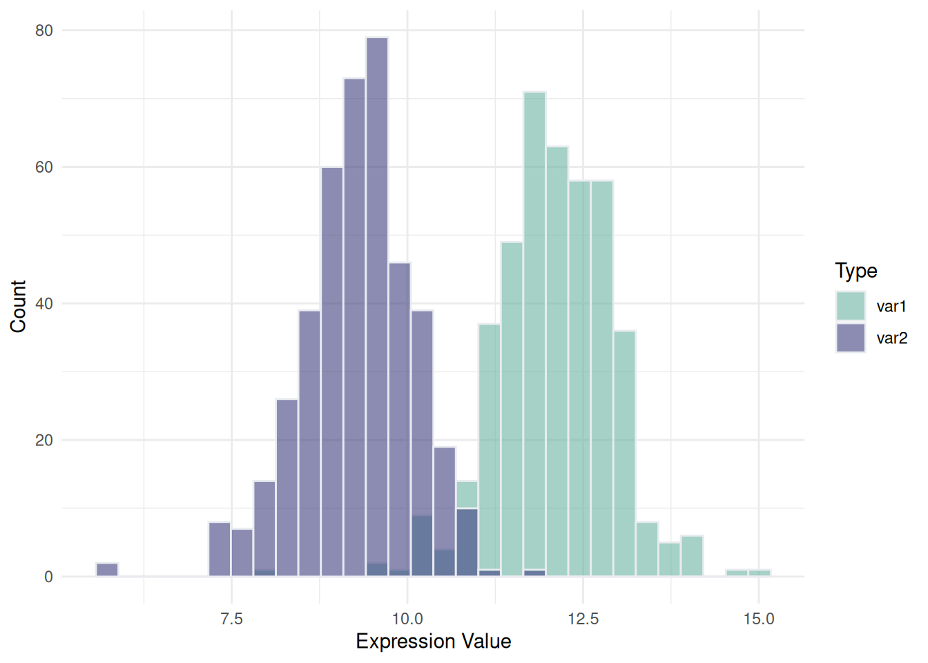
为了更加清晰地比较多个分布的距离,可以统计mean或者median,并绘制密度和垂直线。
p <- data12 %>%
  gghistogram(x = "expression",
   color = "var",
   fill = "var",
   add = "median", # 可以是 mean 或 median
   rug = TRUE,
   palette = c("#00AFBB", "#E7B800")) +
  theme_minimal()

p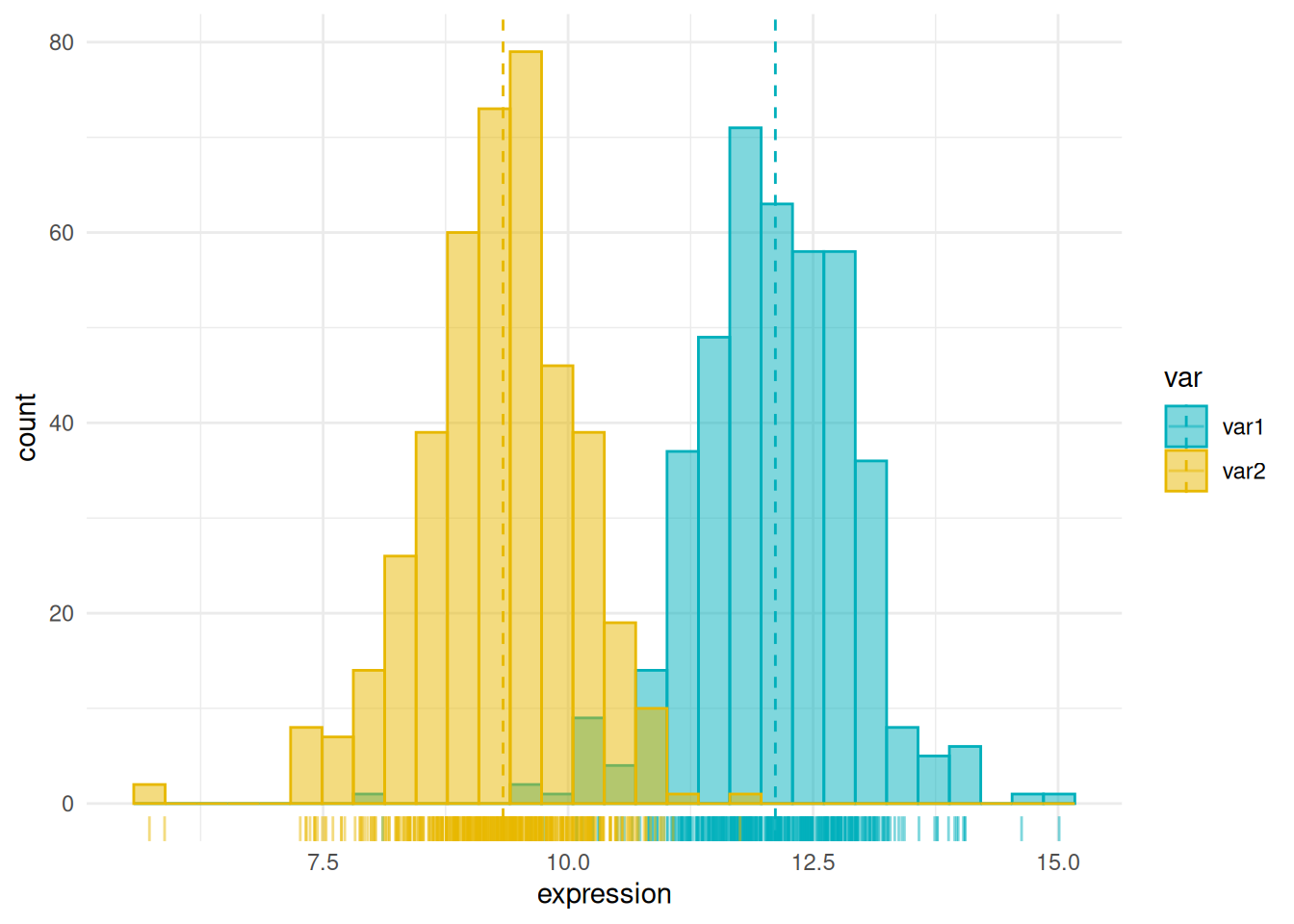
5. 多个变量的分面直方图
分面直方图通过将多个变量或分类变量按面板布局展示,可以实现多维数据的对比、分层和详细分析。相比基础直方图,它不仅在处理复杂数据上更高效,还能避免图形重叠,并提供了更直观的变量对比,尤其在分类变量、分组数据和多变量分析中更具优势。
# 使用内置 iris 数据集
data <- iris

# 将数据从宽格式重塑为长格式
data <- data %>%
  gather(key = "variable", value = "value", -Species)  # 排除Species列

# 绘制分面直方图
p <- data %>%
  ggplot(aes(x = value, color = Species, fill = Species)) +
  geom_histogram(alpha = 0.6, binwidth = 0.3, position = "identity") +
  scale_fill_viridis(discrete = TRUE, option = "D") +
  scale_color_viridis(discrete = TRUE, option = "D") +
  theme(
    legend.position = "bottom",
    panel.spacing = unit(0.5, "lines"),
    strip.text.x = element_text(size = 10)
  ) +
  xlab("Value") +
  ylab("Frequency") +
  facet_grid(Species ~ variable, scales = "free_x")  # 创建分面网格

p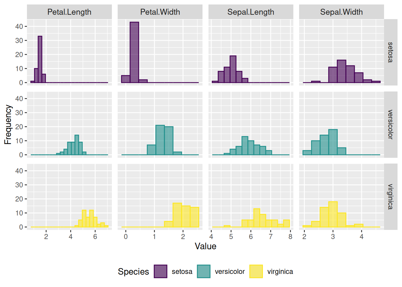
6. 使用 ggMarginal() 添加边际分布
# 使用边际直方图创建散点图
p <- ggplot(mtcars, aes(x = wt, y = mpg, color = factor(cyl), size = factor(cyl))) +
  geom_point(aes(color = factor(cyl)), show.legend = TRUE) +  # 散点图根据 cyl 变化大小
  geom_smooth(method = 'lm', formula = y ~ x, se = TRUE, linewidth = 1, aes(color = factor(cyl))) +  # 回归曲线
  scale_color_manual(values = c("#2e3b97", "#faad61", "#b76252")) +  # 指定回归曲线颜色
  stat_regline_equation(
    aes(label = paste(after_stat(eq.label), after_stat(rr.label), sep = "~~~~")),
    formula = y ~ x, size = 3,
    position = position_nudge(x = 2.7, y = 1)
  ) +  # 添加回归方程和 R² 值
  theme(legend.position = "none")  # 隐藏图例,实现更清晰的可视化

# 向散点图添加边际直方图
p1 <- ggMarginal(p, type = "histogram")

# 显示图表
p1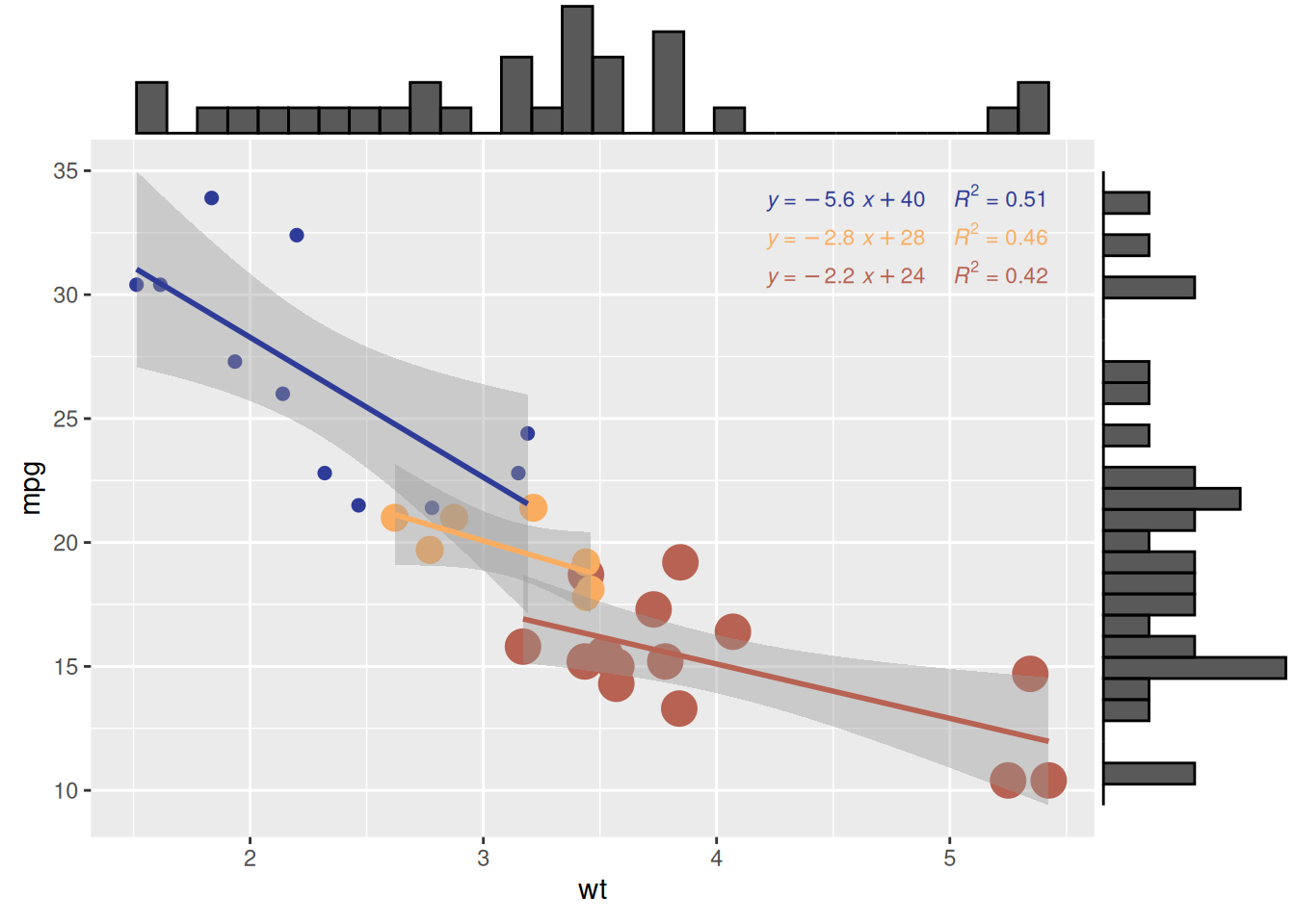
ggMarginal() 添加边际分布
提示
自定义参数用于绘制边际分布图
-
size:改变边际图大小。 - 用常用参数自定义边际图外观。
-
margins = 'x'或margins = 'y':仅显示一个边际图。
# 使用边际直方图创建散点图
p <- ggplot(mtcars, aes(x = wt, y = mpg, color = factor(cyl), size = factor(cyl))) +
  geom_point(aes(color = factor(cyl)), show.legend = TRUE) +  # 散点颜色映射
  geom_smooth(method = 'lm', formula = y ~ x, se = TRUE, linewidth = 1, aes(color = factor(cyl))) +  # 回归曲线
  scale_color_manual(values = c("#2e3b97", "#faad61", "#b76252")) +  # 回归线的自定义颜色
  stat_regline_equation(
    aes(label = paste(after_stat(eq.label), after_stat(rr.label), sep = "~~~~")),
    formula = y ~ x, size = 1.5,
    position = position_nudge(x = 2.2, y = 1)
  ) +  # 添加回归方程和 R² 值
  theme(legend.position = "none")  # 隐藏图例,实现更清晰的可视化

# 更改边际图的大小
p1 <- ggMarginal(p, type = "histogram", size = 10)

# 自定义边际图的外观
p2 <- ggMarginal(p, type = "histogram", fill = "slateblue", xparams = list(bins = 10))

# 仅显示一个边际图(x 轴边际图)
p3 <- ggMarginal(p, type = "histogram", margins = 'x')

cowplot::plot_grid(p1, p2, p3)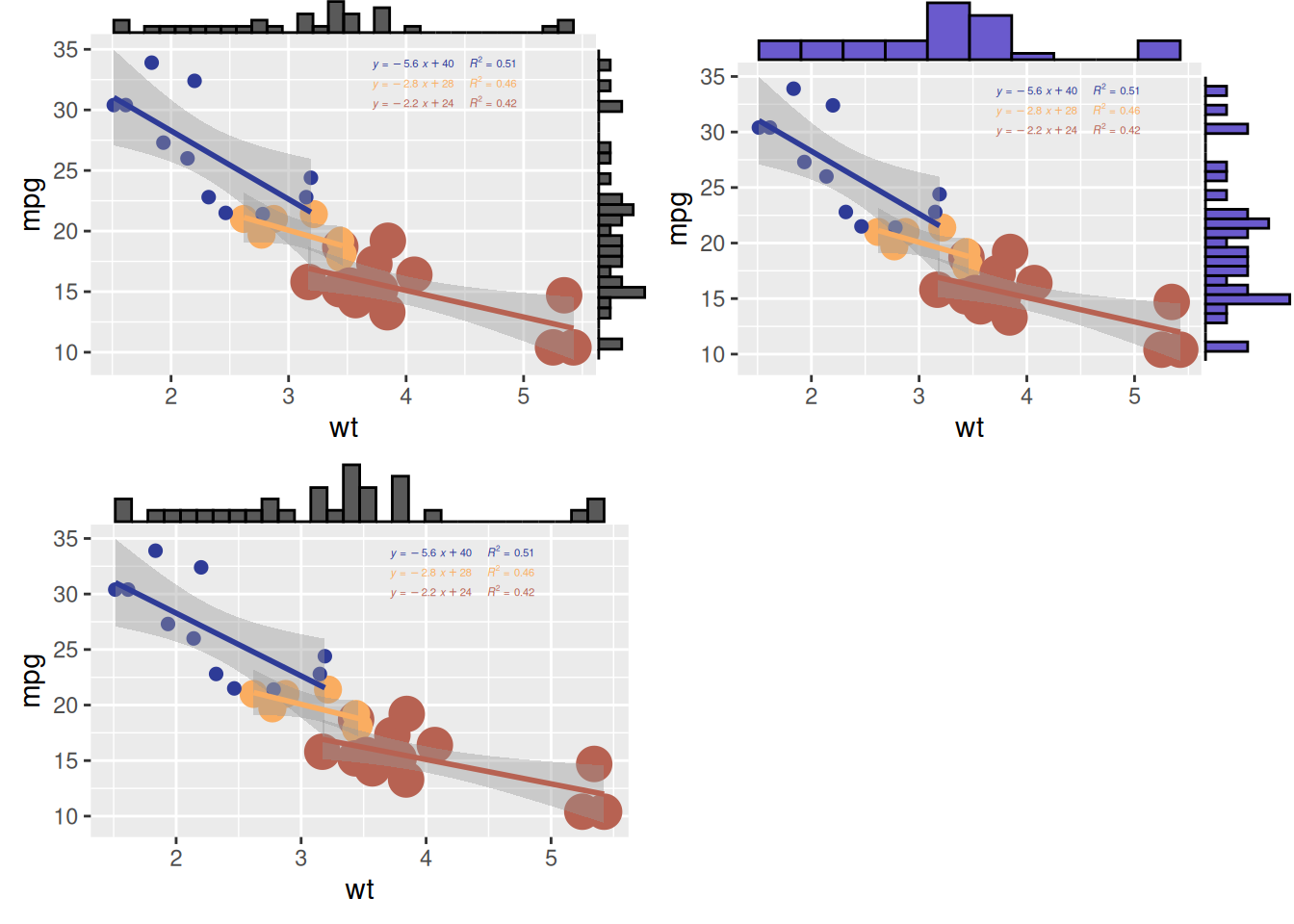
应用场景
1. 基础直方图
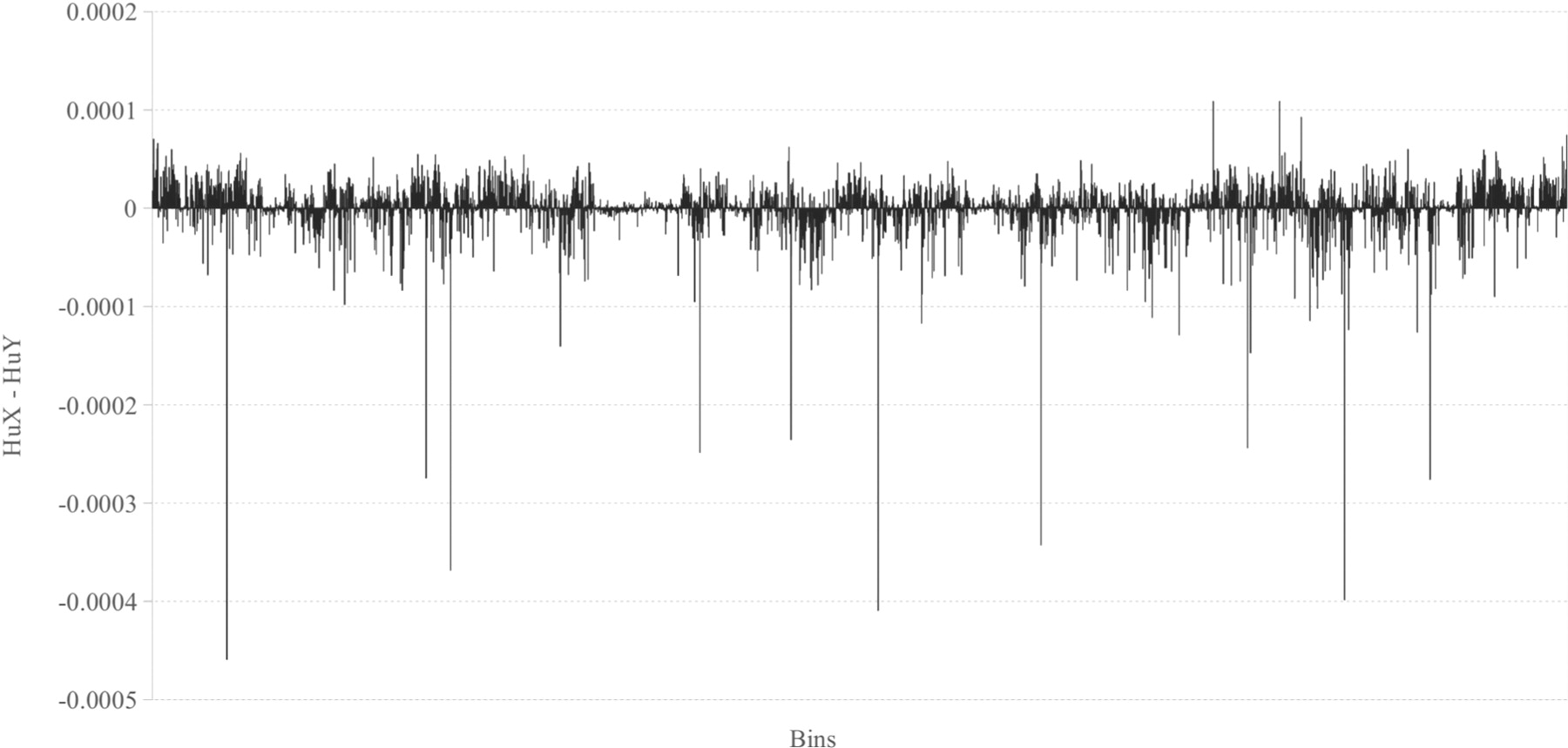
Figure 9 显示了n=6时人类 X 染色体和人类 Y 染色体直方图的相对频率之间的差异。[1]
2. 分面直方图
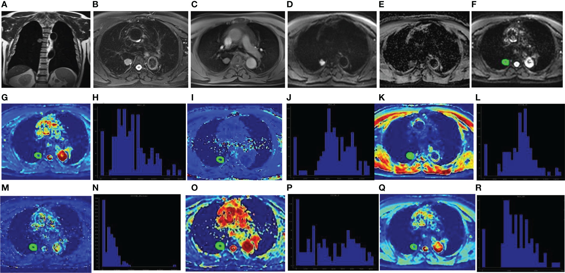
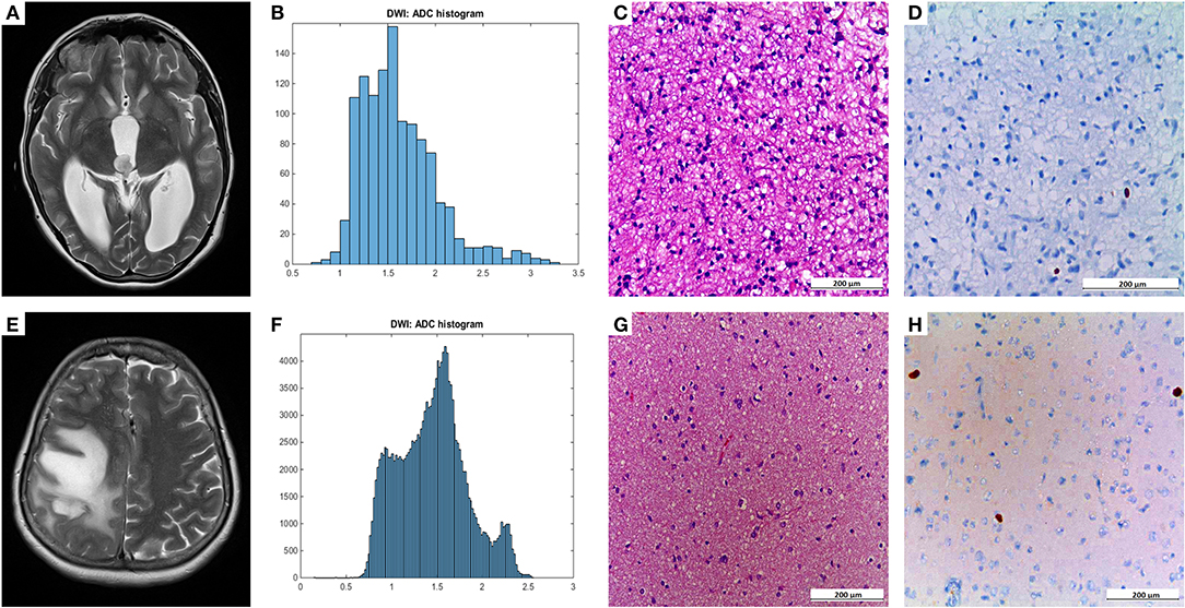
Fig. 10a 显示了典型SPL的影像学表现及病变整体直方图分析如图2所示。[2]
Fig. 10b 展示了 WHO I 级(上排)和 WHO II 级星形细胞瘤(下排)患者的头颅 MRI 示例,包括相应的整个肿瘤 ADC 直方图、H&E 染色和 Ki-67 免疫组织化学结果。 [3]
参考文献
- Costa, A. M., Machado, J. T., & Quelhas, M. D. (2011). Histogram-based DNA analysis for the visualization of chromosome, genome, and species information. Bioinformatics, 27(9), 1207–1214. https://doi.org/10.1093/bioinformatics/btr131
- Xiang, L., Yang, H., Qin, Y., Wen, Y., Liu, X., & Zeng, W.-B. (2023). Differential value of diffusion kurtosis imaging and intravoxel incoherent motion in benign and malignant solitary pulmonary lesions. Frontiers in Oncology, 12, Article 1075072. https://doi.org/10.3389/fonc.2022.1075072
- Gihr, G. A., Horvath-Rizea, D., Hekeler, E., Ganslandt, O., Henkes, H., Hoffmann, K.-T., Scherlach, C., & Schob, S. (2020). Histogram analysis of diffusion weighted imaging in low-grade gliomas: in vivo characterization of tumor architecture and corresponding neuropathology. Frontiers in Oncology, 10, 206. https://doi.org/10.3389/fonc.2020.00206
- Wickham, H., Hester J, & Bryan J. (2024). readr: Read Rectangular Text Data. https://CRAN.R-project.org/package=readr
- Wickham, H. (2016). ggplot2: Elegant graphics for data analysis. Springer. https://ggplot2.tidyverse.org
- Gao, Y. (2021). ggExtra: Add marginal plots to ggplot2. https://cran.r-project.org/package=ggExtra
- Wickham, H., & RStudio Team. (2019). tidyverse: Easily install and load the ‘tidyverse’. https://cran.r-project.org/package=tidyverse
- Claus O. Wilke. (2024). cowplot: Streamlined Plot Theme and Plot Annotations for ‘ggplot2’. https://CRAN.R-project.org/package=cowplot
- García, M. (2018). viridis: Default color maps from ‘matplotlib’. https://cran.r-project.org/package=viridis
- Aubry, R., & Bouchard, C. (2020). ggpmisc: Miscellaneous extensions to ‘ggplot2’. https://cran.r-project.org/package=ggpmisc
- Kassambara, A. (2021). ggpubr: ‘ggplot2’ based publication-ready plots. https://cran.r-project.org/package=ggpubr