import matplotlib.pyplot as plt
import pandas as pd
import numpy as np火山图(Python)
火山图同时显示统计显著性(-log10 p 值)和倍数变化(log2 FC),用于展示数千个特征的差异分析结果。在生物医学研究中,火山图是 RNA-seq、蛋白质组学和代谢组学差异基因表达结果的标准可视化方式。Python 的 matplotlib 可以完全自定义这些发表级别的图表。
示例

环境配置
- 系统要求:跨平台(Linux/MacOS/Windows)
- 编程语言:Python
- 依赖包:
matplotlib、pandas、numpy
数据准备
np.random.seed(42)
n_genes = 5000
df = pd.DataFrame({
    'gene': [f'Gene{i+1}' for i in range(n_genes)],
    'log2FC': np.random.normal(0, 1.5, n_genes),
    'pvalue': np.random.uniform(1e-10, 1, n_genes)
})
df['neg_log10p'] = -np.log10(df['pvalue'])

fc_thresh = 1.0
p_thresh = 0.05

conditions = [
    (df['log2FC'] > fc_thresh) & (df['pvalue'] < p_thresh),
    (df['log2FC'] < -fc_thresh) & (df['pvalue'] < p_thresh),
]
choices = ['Up', 'Down']
df['regulation'] = np.select(conditions, choices, default='NS')
可视化
基础火山图
colors = {'Up': '#e63946', 'Down': '#457b9d', 'NS': '#cccccc'}
fig, ax = plt.subplots(figsize=(8, 6))
for reg, color in colors.items():
    subset = df[df['regulation'] == reg]
    ax.scatter(subset['log2FC'], subset['neg_log10p'],
               c=color, s=8, alpha=0.6, label=f'{reg} ({len(subset)})')
ax.axhline(-np.log10(p_thresh), color='grey', linestyle='--', linewidth=0.8)
ax.axvline(fc_thresh, color='grey', linestyle='--', linewidth=0.8)
ax.axvline(-fc_thresh, color='grey', linestyle='--', linewidth=0.8)
ax.set_xlabel('log₂(Fold Change)')
ax.set_ylabel('-log₁₀(P-value)')
ax.set_title('Volcano Plot')
ax.legend(frameon=False)
ax.spines[['top', 'right']].set_visible(False)
plt.tight_layout()
plt.show()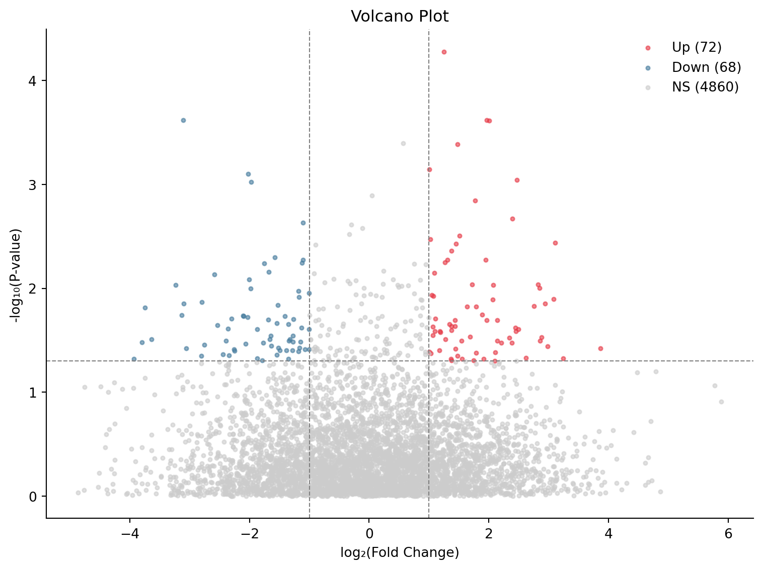
带基因标签的火山图
fig, ax = plt.subplots(figsize=(9, 7))
for reg, color in colors.items():
    subset = df[df['regulation'] == reg]
    ax.scatter(subset['log2FC'], subset['neg_log10p'],
               c=color, s=8, alpha=0.5, label=f'{reg} ({len(subset)})')

top_genes = df.nlargest(15, 'neg_log10p')
for _, row in top_genes.iterrows():
    ax.annotate(row['gene'], (row['log2FC'], row['neg_log10p']),
                fontsize=7, ha='center', va='bottom',
                arrowprops=dict(arrowstyle='-', color='grey', lw=0.5))

ax.axhline(-np.log10(p_thresh), color='grey', linestyle='--', linewidth=0.8)
ax.axvline(fc_thresh, color='grey', linestyle='--', linewidth=0.8)
ax.axvline(-fc_thresh, color='grey', linestyle='--', linewidth=0.8)
ax.set_xlabel('log₂(Fold Change)')
ax.set_ylabel('-log₁₀(P-value)')
ax.set_title('Volcano Plot with Top Gene Labels')
ax.legend(frameon=False, loc='upper left')
ax.spines[['top', 'right']].set_visible(False)
plt.tight_layout()
plt.show()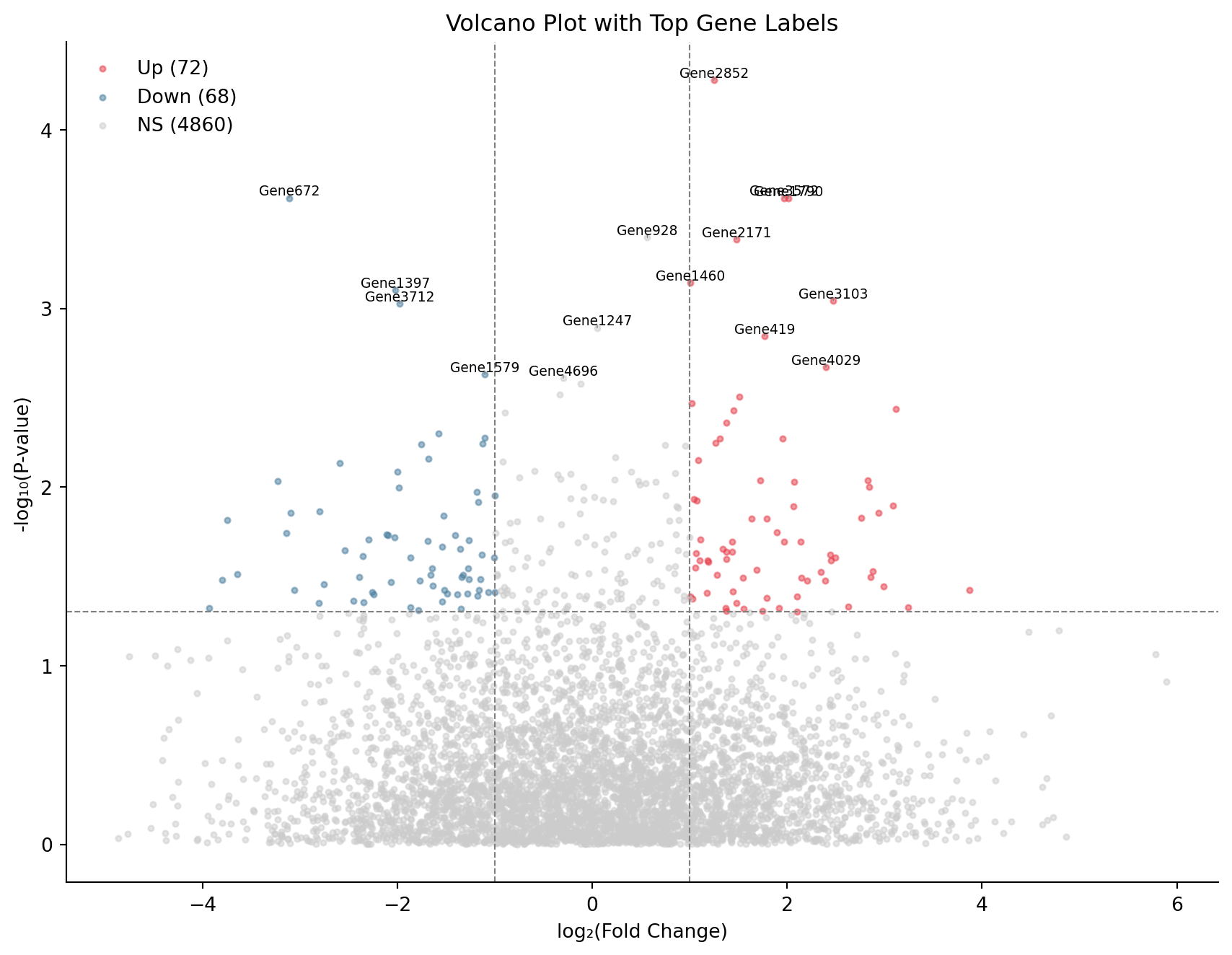
增强火山图
fig, ax = plt.subplots(figsize=(9, 7))
sig_up = df[(df['regulation'] == 'Up')]
sig_down = df[(df['regulation'] == 'Down')]
ns = df[df['regulation'] == 'NS']

ax.scatter(ns['log2FC'], ns['neg_log10p'], c='#e0e0e0', s=6, alpha=0.4, label=f'NS ({len(ns)})')
ax.scatter(sig_down['log2FC'], sig_down['neg_log10p'], c='#457b9d', s=12, alpha=0.7, label=f'Down ({len(sig_down)})')
ax.scatter(sig_up['log2FC'], sig_up['neg_log10p'], c='#e63946', s=12, alpha=0.7, label=f'Up ({len(sig_up)})')

ax.axhline(-np.log10(p_thresh), color='black', linestyle=':', linewidth=0.8, alpha=0.5)
ax.axvline(fc_thresh, color='black', linestyle=':', linewidth=0.8, alpha=0.5)
ax.axvline(-fc_thresh, color='black', linestyle=':', linewidth=0.8, alpha=0.5)
ax.fill_betweenx([0, df['neg_log10p'].max()], fc_thresh, df['log2FC'].max(),
                 alpha=0.03, color='red')
ax.fill_betweenx([0, df['neg_log10p'].max()], df['log2FC'].min(), -fc_thresh,
                 alpha=0.03, color='blue')
ax.set_xlabel('log₂(Fold Change)', fontsize=12)
ax.set_ylabel('-log₁₀(P-value)', fontsize=12)
ax.set_title('Enhanced Volcano Plot', fontsize=14)
ax.legend(frameon=True, fancybox=True, shadow=True)
ax.spines[['top', 'right']].set_visible(False)
plt.tight_layout()
plt.show()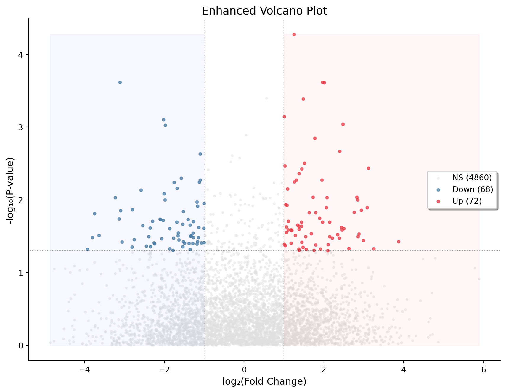
参考文献
- Li, W. (2012). Volcano plots in analyzing differential expressions with mRNA microarrays. Journal of Bioinformatics and Computational Biology, 10(6), 1231003.