# 安装必要的包
if (!requireNamespace("tidycmprsk", quietly = TRUE)) {
  install.packages("tidycmprsk")
}
if (!requireNamespace("ggsurvfit", quietly = TRUE)) {
  install.packages("ggsurvfit")
}

# 加载包
library(survival)
library(tidycmprsk)
library(ggsurvfit)
library(ggplot2)
library(dplyr)竞争风险累积发生曲线
当患者可能死于多种原因——进展或死亡、复发或移植相关死亡——对目标事件做标准 Kaplan–Meier 分析是错误的:把发生竞争事件的患者当作删失,等于假设他们仍有进展风险,于是朴素的 1−KM 估计量会高估发生率;竞争事件越常见,高估越严重 [1]。正确的描述工具是累积发生函数(CIF,Aalen–Johansen 估计量),它把竞争事件视为竞争:死亡的患者不再可能进展,所有病因的 CIF 之和为 1。
组间比较用 Gray 检验(对 CIF 的 K 样本检验),回归用 Fine–Gray 分布下风险模型 [2]。本教程用 tidycmprsk [3] 与 ggsurvfit [4] 在经典 mgus2 队列 [5] 上演示全部三项:1,384 例意义未明单克隆丙种球蛋白病(MGUS)患者,进展为浆细胞恶性肿瘤(PCM)与死亡互为竞争风险。
本教程涵盖四种工作流:
- 两个竞争结局的 CIF(含置信区间与风险表);
- 按协变量分组的 CIF 与 Gray 检验;
- Fine–Gray 分布下风险回归;
- 1−KM 为何高估发生率——审稿人必问的对比图。
Example
Setup
系统要求:跨平台(Linux/MacOS/Windows)
编程语言:R
依赖包:
survival;tidycmprsk;ggsurvfit;ggplot2;dplyr
sessioninfo::session_info("attached")─ Session info ───────────────────────────────────────────────────────────────
setting value
version R version 4.6.2 (2026-10-29)
os Ubuntu 24.04.5 LTS
system x86_64, linux-gnu
ui X11
language (EN)
collate C.UTF-8
ctype C.UTF-8
tz UTC
date 2026-10-31
pandoc 3.1.3 @ /usr/bin/ (via rmarkdown)
quarto 1.10.20 @ /usr/local/bin/quarto
─ Packages ───────────────────────────────────────────────────────────────────
! package * version date (UTC) lib source
P dplyr * 1.2.1 2026-04-03 [?] RSPM
P ggplot2 * 4.0.3.9000 2026-10-30 [?] Github (tidyverse/ggplot2@b638d65)
ggsurvfit * 1.2.1 2026-07-24 [1] RSPM
P survival * 3.8-6 2026-01-16 [?] RSPM
tidycmprsk * 1.1.2 2026-04-09 [1] RSPM
[1] /home/runner/.cache/R/renv/library/Bizard-5140bdc6/linux-ubuntu-noble/R-4.6/x86_64-pc-linux-gnu
[2] /home/runner/work/_temp/Library
[3] /opt/R/4.6.2/lib/R/library
* ── Packages attached to the search path.
P ── Loaded and on-disk path mismatch.
──────────────────────────────────────────────────────────────────────────────Data Preparation
mgus2 随 survival 包发布 [5]:1,384 例 MGUS 患者自诊断起随访,观察进展为浆细胞恶性肿瘤(PCM)或死亡。随访时间取进展时间(ptime)与末次接触(futime)的较早者;竞争风险事件编码 0 = 删失、1 = PCM(目标事件)、2 = 死亡(竞争事件)。
data(mgus2)

mgus2$etime <- with(mgus2, ifelse(pstat == 1, ptime, futime))
mgus2$event <- with(mgus2, ifelse(pstat == 1, 1, ifelse(death == 1, 2, 0)))
mgus2$event_f <- factor(mgus2$event, levels = 0:2,
                        labels = c("censored", "pcm", "death"))

cat("Patients:", nrow(mgus2),
    "| progression:", sum(mgus2$event == 1),
    "| death (competing):", sum(mgus2$event == 2), "\n")
Patients: 1384 | progression: 115 | death (competing): 860 Visualization
1. 两个结局的累积发生率
ci1 <- cuminc(Surv(etime, event_f) ~ 1, data = mgus2)

ggcuminc(ci1, outcome = c("pcm", "death")) +
  add_confidence_interval() +
  add_risktable(size = 3) +
  scale_color_manual(values = c(pcm = "#B2182B", death = "#2166AC"), name = NULL) +
  scale_fill_manual(values = c(pcm = "#B2182B", death = "#2166AC"), guide = "none") +
  xlab("Months since diagnosis") +
  ylab("Cumulative incidence") +
  theme_bw(base_size = 11)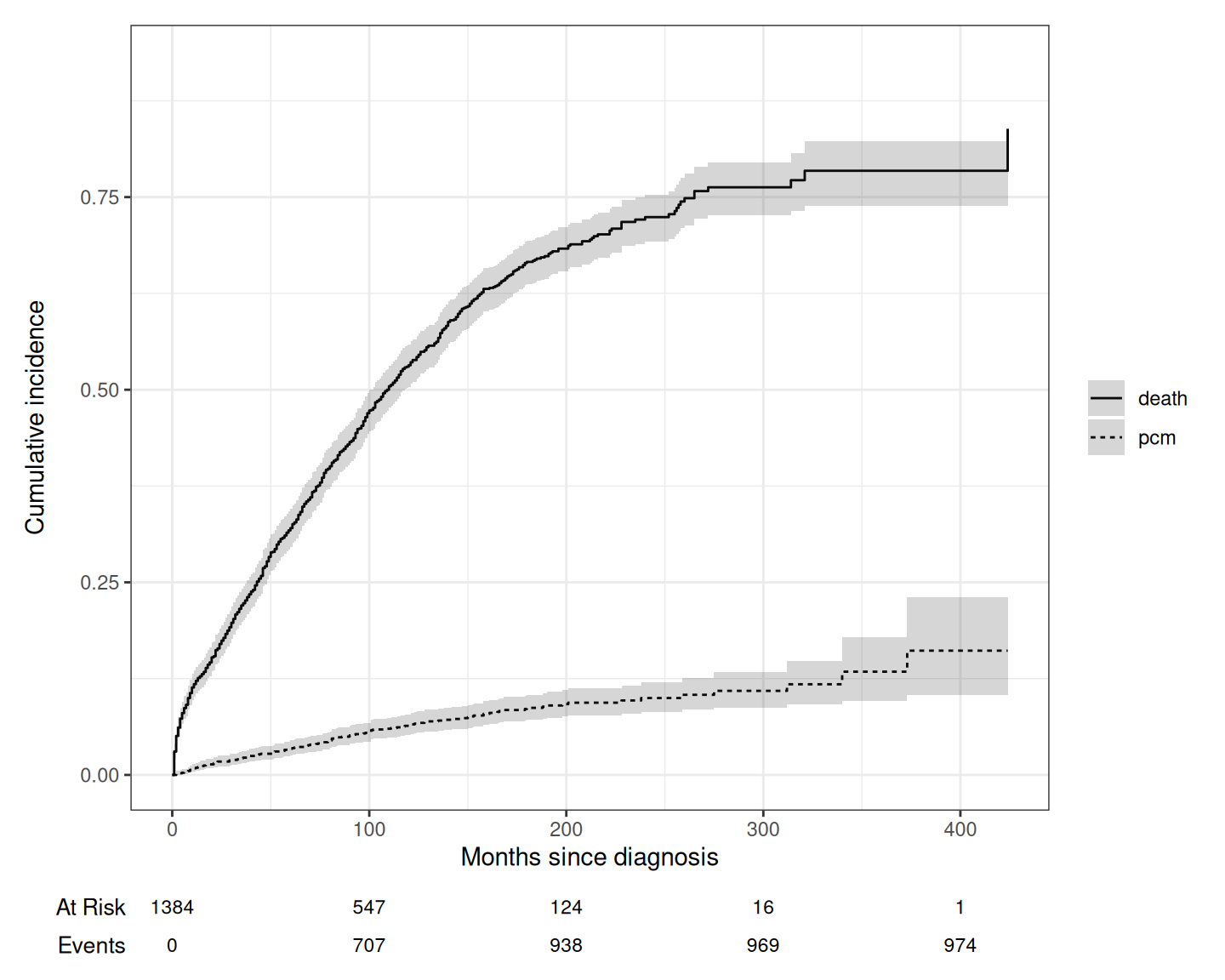
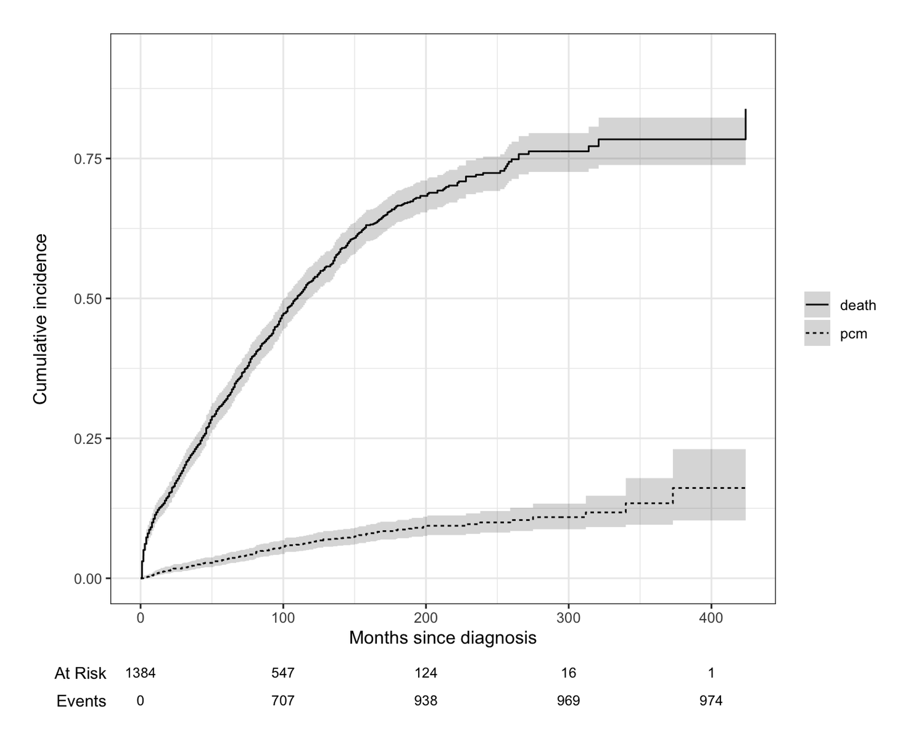
死亡占主导:到 20 年约 78% 死亡、仅约 16% 进展——这正是朴素 Kaplan–Meier 分析进展率会出错的场景(见第 4 节)。
2. 用 Gray 检验比较分组
ci2 <- cuminc(Surv(etime, event_f) ~ sex, data = mgus2)
gt <- glance(ci2)
cat(sprintf("Gray's test, progression: chi-square = %.2f, df = %d, p = %.3f\n",
            gt$statistic_1, gt$df_1, gt$p.value_1))
Gray's test, progression: chi-square = 1.19, df = 1, p = 0.274cat(sprintf("Gray's test, death: chi-square = %.2f, df = %d, p = %.3f\n",
gt$statistic_2, gt$df_2, gt$p.value_2))Gray's test, death: chi-square = 11.65, df = 1, p = 0.001ggcuminc(ci2, outcome = "pcm") +
add_confidence_interval() +
scale_color_manual(values = c(F = "#1B9E77", M = "#7570B3"), name = "Sex") +
scale_fill_manual(values = c(F = "#1B9E77", M = "#7570B3"), guide = "none") +
xlab("Months since diagnosis") +
ylab("Cumulative incidence of progression") +
theme_bw(base_size = 11)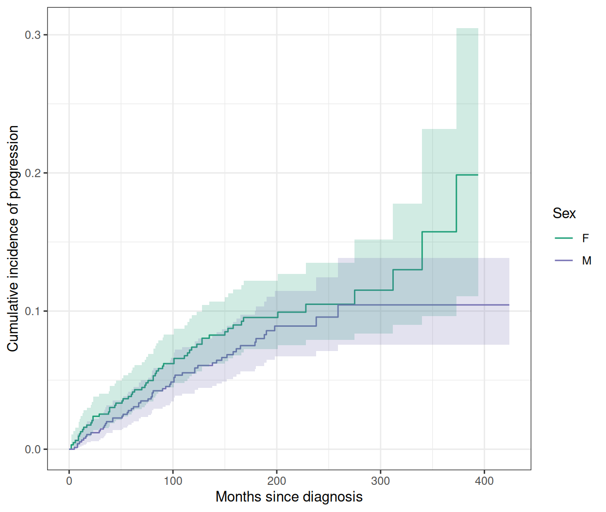
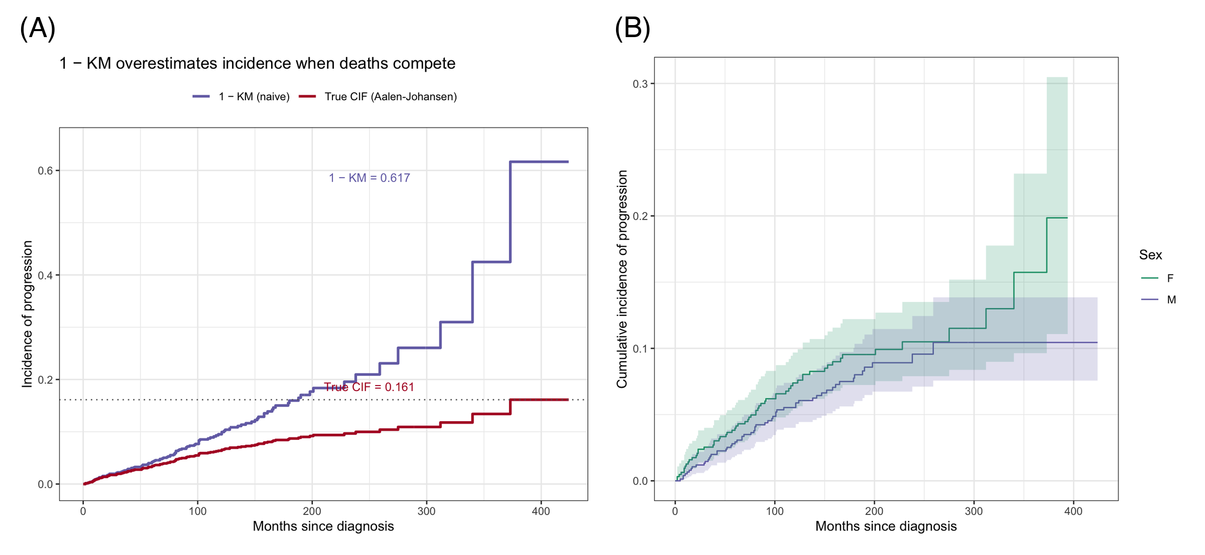
男性进展略快于女性,但 Gray 检验未达 0.05 显著水平——效应量由下方的回归恰当地量化。
3. Fine–Gray 回归
fg <- crr(Surv(etime, event_f) ~ sex + age, data = mgus2, failcode = "pcm")
fgdf <- tidy(fg, exponentiate = TRUE, conf.int = TRUE) |>
  mutate(term_lbl = recode(term, sexM = "Sex: M vs F", age = "Age (per year)"))

ggplot(fgdf, aes(x = estimate, y = term_lbl)) +
  geom_errorbar(aes(xmin = conf.low, xmax = conf.high), orientation = "y",
                width = 0.12, color = "#B2182B") +
  geom_point(size = 3, color = "#B2182B") +
  geom_vline(xintercept = 1, linetype = "dashed", color = "grey40") +
  scale_x_log10() +
  labs(x = "Subdistribution hazard ratio (log scale)", y = NULL,
       title = "Fine-Gray regression: progression to malignancy") +
  theme_bw(base_size = 11)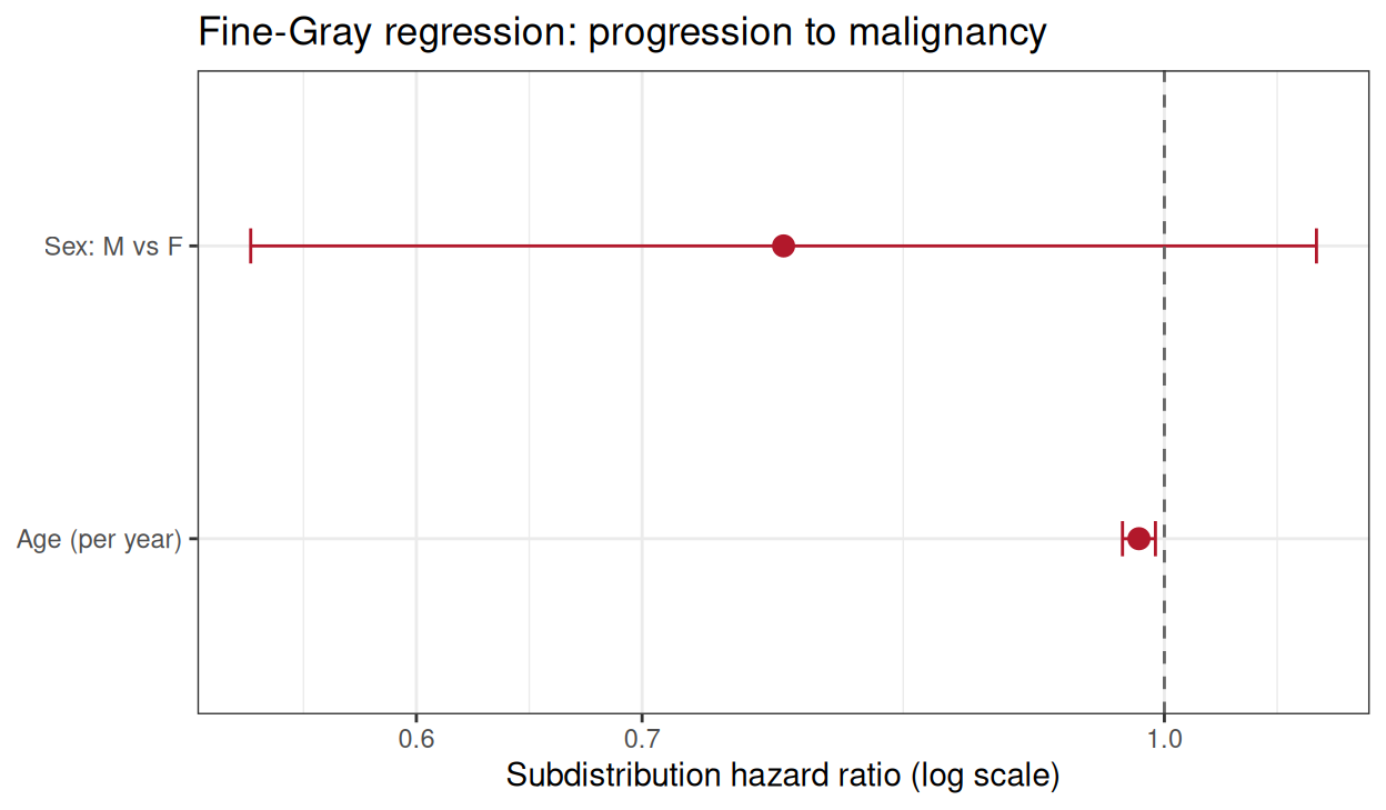
分布下风险 HR 回答的是临床相关问题——协变量如何移动竞争风险存在下的进展绝对发生率。若研究病因学(cause-specific)问题,改用 survival::coxph 并在报告中说明用的是哪一种。
4. 1−KM 为何高估:对比图
kmfit <- survfit(Surv(etime, event == 1) ~ 1, data = mgus2)  # 死亡作删失
kmdf <- data.frame(time = kmfit$time, est = 1 - kmfit$surv)
cidf <- tidy(ci1) |>
  filter(outcome == "pcm") |>
  select(time, cif = estimate)
cidf <- rbind(data.frame(time = 0, cif = 0), cidf)

ggplot() +
  geom_step(data = kmdf, aes(time, est, color = "1 − KM (naive)"),
            linewidth = 1, direction = "hv") +
  geom_step(data = cidf, aes(time, cif, color = "True CIF (Aalen-Johansen)"),
            linewidth = 1, direction = "hv") +
  geom_hline(yintercept = tail(cidf$cif, 1), linetype = "dotted", color = "grey40") +
  annotate("text", x = 250, y = tail(cidf$cif, 1) + 0.025, size = 3.4, color = "#B2182B",
           label = sprintf("True CIF = %.3f", tail(cidf$cif, 1))) +
  annotate("text", x = 250, y = max(kmdf$est) - 0.03, size = 3.4, color = "#7570B3",
           label = sprintf("1 − KM = %.3f", max(kmdf$est))) +
  scale_color_manual(values = c("1 − KM (naive)" = "#7570B3",
                                "True CIF (Aalen-Johansen)" = "#B2182B"), name = NULL) +
  coord_cartesian(xlim = c(0, 420), ylim = c(0, 0.65)) +
  labs(x = "Months since diagnosis", y = "Incidence of progression",
       title = "1 − KM overestimates incidence when deaths compete") +
  theme_bw(base_size = 11) + theme(legend.position = "top")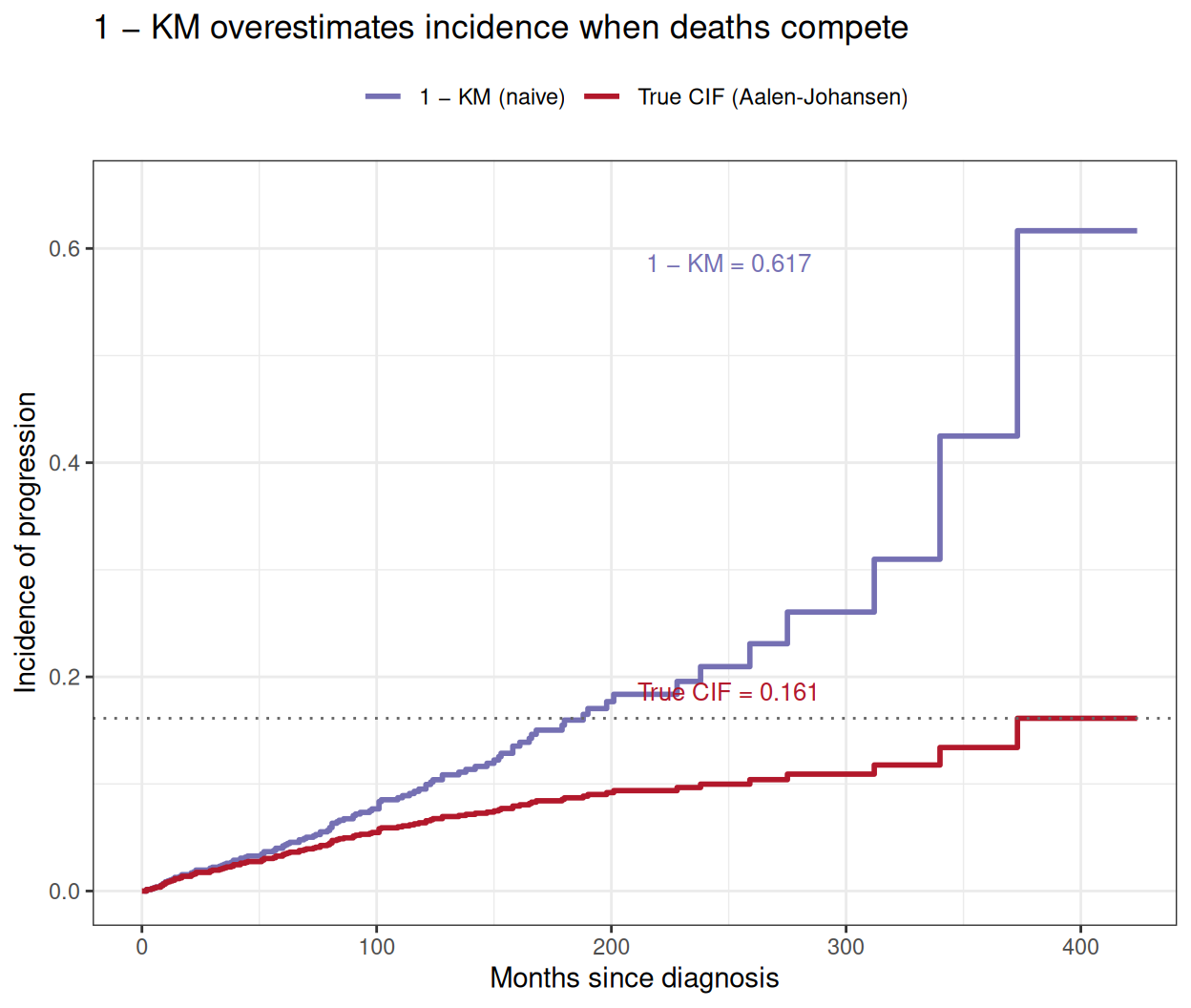
朴素曲线在 20 年时比真实值高出近四倍。只要竞争事件不罕见,就应报告 Aalen–Johansen CIF——只画目标事件的 Kaplan–Meier 曲线是审稿中常见且后果严重的错误。
提示实践要点
- 结局编码为因子,目标事件在前、竞争事件次之、删失最后;
tidycmprsk::cuminc()需要两水平Surv(time, factor)语法。 - 报告 CIF 时附置信区间与风险表——读者判断的是随访质量,不只是曲线。
- Gray 检验比较发生率;对 cause-specific 生存做 log-rank 回答的是另一个问题。按估计目标选择。
- Fine–Gray 模型中协变量对分布下风险的效应符号可能反直觉(年龄显得”保护性”,因为死亡先移除了患者)——对照 CIF 而非风险解读。
Application
竞争风险曲线是移植(复发 vs 非复发死亡)、老年肿瘤(进展 vs 其他原因死亡)与器械/心脏病研究(心律失常 vs 全因死亡)的标准图表。下图模拟典型论文版式:(A) 两个结局的 CIF 与风险表,(B) 朴素 1−KM 与真实 CIF 对比。
Reference
[1] Austin PC, Fine JP. Practical recommendations for reporting Fine-Gray model analyses for competing risk data. Stat Med. 2017;36(4):5391-5400. doi:10.1002/sim.7501
[2] Fine JP, Gray RJ. A proportional hazards model for the subdistribution of a competing risk. J Am Stat Assoc. 1999;94(446):496-509. doi:10.1080/01621459.1999.10474144
[3] Sjoberg DD, Fei T. tidycmprsk: competing risks estimation. R package version 1.1.2. 2026. doi:10.32614/CRAN.package.tidycmprsk
[4] Sjoberg DD, Whiting K, Curry M, Lavery JA, Larmarange J. Reproducible summary tables with the gtsummary package. R J. 2021;13:570-580. doi:10.32614/RJ-2021-053 (ggsurvfit builds on gtsummary)
[5] Kyle RA, Therneau TM, Rajkumar SV, et al. A long-term study of prognosis in monoclonal gammopathy of undetermined significance. N Engl J Med. 2002;346(8):564-569. doi:10.1056/NEJMoa011332